
|
|
|
|||||||
followed by the augmented functional
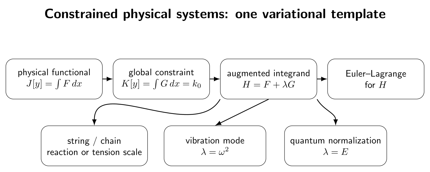
where the multiplier λ is constant for a single scalar integral constraint. In physical applications, that multiplier often has an additional interpretation: it may act like a reaction load, a horizontal Tension scale, a squared natural frequency, an energy eigenvalue, or a generalized force associated with the imposed global condition. This is one reason constrained variational methods are so useful across mechanics and physics [1, 2, 3].
Figure. The same constrained-variation template appears in apparently different physical systems. The multiplier is introduced mathematically to enforce the integral constraint; its physical interpretation depends on the problem.
1 Exercises
Exercise 1: taut string with prescribed mean deflectionA taut string on 0 ≤ x ≤ L has constant tension T and fixed endpoints
Its small-slope elastic energy is
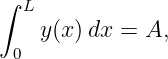
Among all admissible shapes satisfying the prescribed area/mean-deflection condition
find the stationary shape and determine the multiplier. Then evaluate the minimum energy.
Exercise 2: string on an elastic foundation with prescribed mean deflectionLet
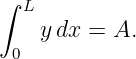
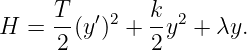
with T > 0, k > 0, and y(0) = y(L) = 0. Impose
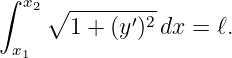
Exercise 3: the hanging chain as a fixed-length constrained systemA uniform flexible chain with Weight per unit arc length w hangs in a uniform gravitational field. Its endpoints are fixed horizontally, and its total length is prescribed:
Take the vertical coordinate y positive upward. The gravitational potential energy is
Exercise 4: normalized vibration mode of a uniform stringA uniform string of mass density μ and tension T is fixed at x = 0 and x = L. Minimize the strain-energy functional
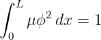
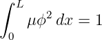
subject to the normalization
and endpoint conditions ϕ(0) = ϕ(L) = 0.
Exercise 5: variable-density string as a Sturm–Liouville problemLet T(x) > 0 and μ(x) > 0. Minimize
subject to
Derive the differential equation and explain why the multiplier is again an eigenvalue parameter.
Exercise 6: normalization in the one-dimensional infinite square wellFor a real wavefunction ψ(x) on 0 ≤ x ≤ L, consider the kinetic-energy expectation functional
with
Exercise 7: a particle trajectory with a prescribed time integral of positionA particle moves on a line during 0 ≤ t ≤ τ. Consider
with
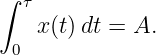
Impose the global trajectory constraint
Find the stationary trajectory and interpret the multiplier as an effective constant generalized force.
Exercise 8: selecting the second string mode with two constraintsFor the same uniform string as Exercise 4, minimize
subject to both
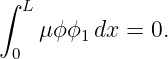
and orthogonality to the normalized fundamental mode ϕ1:
Use two multipliers to derive the stationarity equation and show that the minimizer is the normalized second mode.
2 Solutions
Solution 1: taut string with prescribed mean deflectionThe unconstrained integrand is
and the constraint integrand is simply
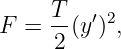
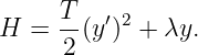
Use
Then
so Euler–Lagrange gives
Thus
Integrating twice,
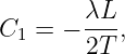
The fixed endpoints give C2 = 0 and
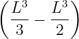
hence
Now impose the global constraint:
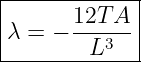
Therefore
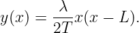
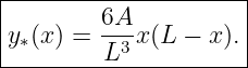
and
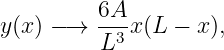
For A > 0, the multiplier is negative in the convention H = F + λG.
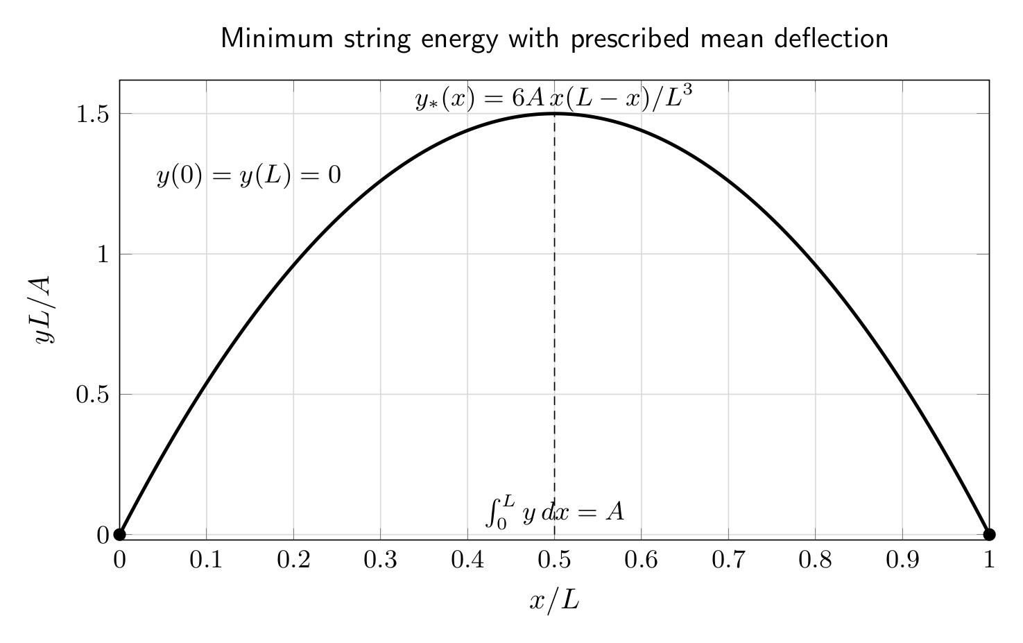
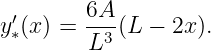
Figure. The minimum-energy string shape under a prescribed integral of displacement is a parabola. The global constraint fixes its amplitude. The derivative is
Therefore
Because the functional is strictly convex in y′ and the constraint is affine, this stationary function is the unique minimizer within the fixed-endpoint admissible class.
Solution 2: elastic foundation plus prescribed mean deflectionThe augmented integrand is
Euler–Lagrange gives
or
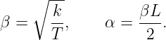
Define
A form that makes the symmetry about L∕2 explicit is
At x = 0 and x = L, the ratio of coshes is one, so the endpoint conditions hold automatically. Integrating,
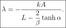
Hence
The denominator is positive, so A > 0 again corresponds to λ < 0. To recover the k → 0 limit, use
Since β2 = k∕T, expansion of the solution and multiplier gives
which is precisely Exercise 1.
Solution 3: hanging chain with fixed lengthThe constrained problem is to minimize gravitational potential energy while keeping the total arc length fixed. The augmented integrand is
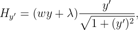
There is no explicit x dependence, so the Beltrami identity gives
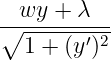
Now
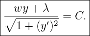
and therefore
Thus
Define
Then
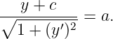
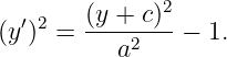
Rearranging,
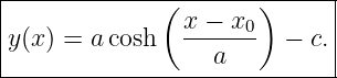
The standard integration gives
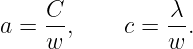
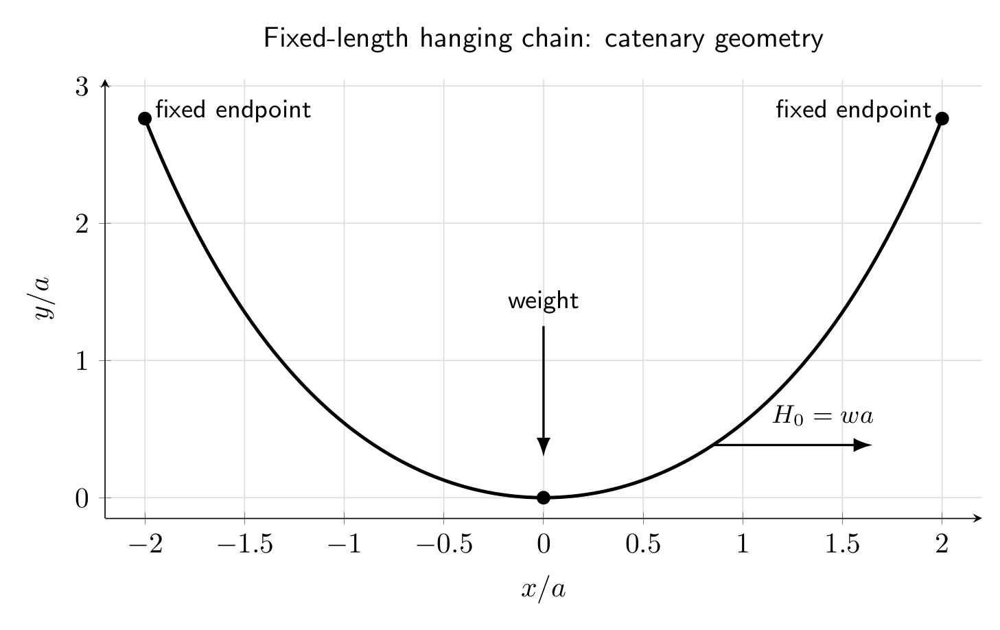
Figure. The fixed-length constraint introduces a multiplier into the potential-energy problem. The Beltrami first integral reduces the resulting equation to the catenary. For a static chain, the horizontal component of the tension is constant. Denoting it by H0, elementary force balance gives the familiar catenary scale
But wa = C from the first integral, so the Beltrami constant is precisely the constant horizontal tension. This is a useful example in which the variational constant has an immediate mechanical interpretation. The catenary and its variational formulation are classical applications of the calculus of variations [2, 1].
Solution 4: normalized vibration mode of a uniform stringUse the augmented functional
The factor 1∕2 is merely convenient. Euler–Lagrange gives
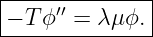
or
For constant T and μ,
The fixed endpoints require
and hence
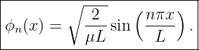
The normalization gives
so
For the physical wave equation
Separation of variables gives
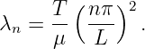
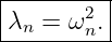
Therefore
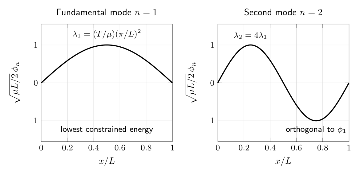
Figure. Normalization removes the arbitrary amplitude of each eigenmode. Among all normalized endpoint-zero functions, the fundamental mode has the smallest strain energy. Multiply the eigenvalue equation by ϕn and integrate. Integration by parts gives
Hence
Because λn ∝ n2, the minimum occurs at n = 1. This variational characterization of vibration modes is a prototype of the Rayleigh quotient and more general eigenvalue principles [4, 5].
Solution 5: variable-density stringUse
Then
Therefore
or
This is a Sturm–Liouville eigenvalue problem with weight μ(x). In the vibration interpretation, λ = ω2. The normalization fixes the eigenfunction scale, while the endpoint conditions and differential equation select the admissible eigenvalues.
Solution 6: normalization in the infinite square wellThe constrained functional is
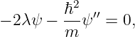
Euler–Lagrange gives
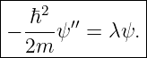
or
This is the time-independent Schrödinger equation inside an infinite square well, with the variational multiplier playing the role of the energy eigenvalue. The boundary conditions give
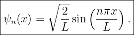
and normalization gives
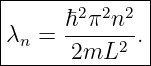
The corresponding multipliers are
To verify that the multiplier equals the energy functional, multiply the differential equation by ψn and integrate:
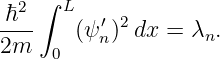
The normalization makes the right side equal to λn. Integrating the left side by parts and using ψn(0) = ψn(L) = 0 gives
Thus
The minimum occurs at n = 1. This is the simplest example of the quantum variational principle with a normalization constraint [6].
Solution 7: constrained particle trajectoryThe augmented integrand is
Euler–Lagrange gives
so
With x(0) = x(τ) = 0,
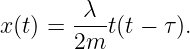
The integral constraint gives
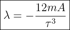
Hence
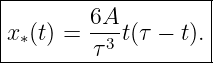
and
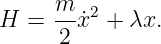
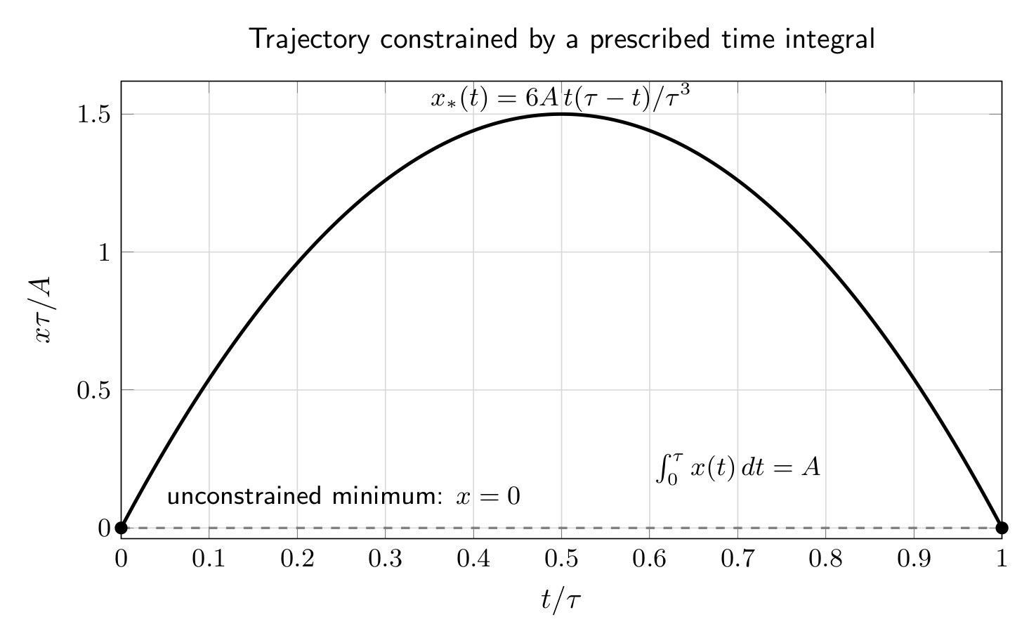
Figure. Without the integral constraint the kinetic functional is minimized by the zero path. Prescribing the time integral of position forces a parabolic trajectory. The equation
has the form of Newton’s law under a constant generalized force. In the convention used here, positive prescribed A requires λ < 0 because the augmented term was chosen as +λx. Reversing the sign convention for the multiplier reverses that sign but not the physical trajectory.
Solution 8: selecting the second string mode with two constraintsIntroduce two multipliers and use
Euler–Lagrange gives
To determine γ, multiply by ϕ1 and integrate. Using integration by parts and the fundamental-mode equation
we obtain
But another integration by parts gives
because of the orthogonality constraint. Therefore
The stationarity equation reduces to the ordinary string eigenproblem
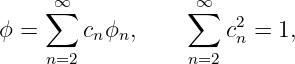
but the extra constraint excludes the fundamental mode. Expanding any admissible normalized function in the orthonormal string modes,
its energy is
Since
the minimum is achieved by placing all weight in the second mode:
This is the basic constrained-minimization mechanism behind variational characterizations of higher eigenmodes: normalization fixes scale, while orthogonality constraints remove lower modes [5, 4].
3 What these physical examples teachThe same mathematical multiplier can play several different physical roles.
The unifying lesson is that a global integral condition changes the set of allowable variations. The multiplier restores the convenience of arbitrary local test functions by transferring the global restriction into the augmented integrand.
4 Common mistakes
5 Bridge to later entriesCV09E2 already points toward several later parts of the series. The string and quantum examples anticipate the variational eigenvalue principles of CV21. The trajectory example connects to Hamilton’s principle in CV14 and optimal control in CV23. The catenary again shows the usefulness of the first-integral methods of CV06. Multiple orthogonality constraints foreshadow systematic constrained-mode and Rayleigh–Ritz calculations. The next main entry, CV10, changes the kind of admissible curve rather than imposing a global integral constraint: stationary paths may be only piecewise smooth, leading to the Weierstrass–Erdmann corner conditions.
References
[1] I. M. Gelfand and S. V. Fomin, Calculus of Variations, Dover Publications, 2000. [2] Cornelius Lanczos, The Variational Principles of Mechanics, 4th ed., Dover Publications, 1986. [3] Herbert Goldstein, Charles Poole, and John Safko, Classical Mechanics, 3rd ed., Addison-Wesley, 2001. [4] Leonard Meirovitch, Elements of Vibration Analysis, 2nd ed., McGraw-Hill, 1986. [5] Richard Courant and David Hilbert, Methods of Mathematical Physics, Volume I, Wiley-Interscience, 1989 reprint. [6] David J. Griffiths and Darrell F. Schroeter, Introduction to Quantum Mechanics, 3rd ed., Cambridge University Press, 2018. "Calculus of Variations: Constrained Physical Systems - Worked Examples" is owned by bloftin.
This object's parent. Cross-references: CV06, Hamilton's principle, Newton's law, position, variational principle, boundary, square, vibration, separation of variables, wave equation, static, amplitude, displacement, particle, parameter, differential equation, functions, mass, catenary, identity, potential energy, unit, Weight, mechanics, force, energy, natural frequency, Tension, scalar, systems, CV09E1, CV09 This is version 1 of Calculus of Variations: Constrained Physical Systems - Worked Examples, born on 2026-10-15. Object id is 1471, canonical name is CalculusOfVariationsConstrainedPhysicalSystemsWorkedExamples. Accessed 5 times total. Classification:
|
|
|
|
Pending Errata and AddendaNone.
|
DiscussionNo messages.
|
Interact |
![[parent]](https://images.physicslibrary.org/images/uparrow.png)
![∫ b ′ ∫ b ′
J[y] = F (x,y,y )dx, K [y] = G (x,y,y )dx = k0,
a a](https://images.physicslibrary.org/cache/objects/1471/make4ht/CalculusOfVariationsConstrainedPhysicalSystemsWorkedExamples0x.png)
![∫
^ b
J [y] = (F + λG )dx,
a](https://images.physicslibrary.org/cache/objects/1471/make4ht/CalculusOfVariationsConstrainedPhysicalSystemsWorkedExamples1x.png)

![∫ L
T- ′ 2
U [y] = 2 0 (y ) dx.](https://images.physicslibrary.org/cache/objects/1471/make4ht/CalculusOfVariationsConstrainedPhysicalSystemsWorkedExamples3x.png)
![∫ [ ]
L T- ′2 k- 2
U[y] = 2 (y ) + 2 y dx,
0](https://images.physicslibrary.org/cache/objects/1471/make4ht/CalculusOfVariationsConstrainedPhysicalSystemsWorkedExamples5x.png)
![∫ x
2 ∘ ------′-2
U [y] = w x y 1 + (y ) dx.
1](https://images.physicslibrary.org/cache/objects/1471/make4ht/CalculusOfVariationsConstrainedPhysicalSystemsWorkedExamples8x.png)

![T ∫ L ′2
U [ϕ] = -- (ϕ ) dx
2 0](https://images.physicslibrary.org/cache/objects/1471/make4ht/CalculusOfVariationsConstrainedPhysicalSystemsWorkedExamples10x.png)
![1∫ L
U [ϕ ] = -- T (x)(ϕ′)2 dx
2 0](https://images.physicslibrary.org/cache/objects/1471/make4ht/CalculusOfVariationsConstrainedPhysicalSystemsWorkedExamples12x.png)

![∫ L 2
E [ψ ] = ℏ--(ψ′)2dx,
0 2m](https://images.physicslibrary.org/cache/objects/1471/make4ht/CalculusOfVariationsConstrainedPhysicalSystemsWorkedExamples14x.png)

![m ∫ τ 2
J[x] = -- ˙x dt
2 0](https://images.physicslibrary.org/cache/objects/1471/make4ht/CalculusOfVariationsConstrainedPhysicalSystemsWorkedExamples16x.png)

![∫ L
U [ϕ] = T- (ϕ ′)2dx
2 0](https://images.physicslibrary.org/cache/objects/1471/make4ht/CalculusOfVariationsConstrainedPhysicalSystemsWorkedExamples19x.png)












![[ ]
λ- cosh-(β-(x-−-L∕2-))
y(x) = k coshα − 1 .](https://images.physicslibrary.org/cache/objects/1471/make4ht/CalculusOfVariationsConstrainedPhysicalSystemsWorkedExamples48x.png)

![[ 1 ∫ L ]
------- cosh (β(x − L∕2 ))dx − L
cosh α 0](https://images.physicslibrary.org/cache/objects/1471/make4ht/CalculusOfVariationsConstrainedPhysicalSystemsWorkedExamples50x.png)

![[ ]
2-
β tanh α − L](https://images.physicslibrary.org/cache/objects/1471/make4ht/CalculusOfVariationsConstrainedPhysicalSystemsWorkedExamples52x.png)



![[ ]
∘ --------- (y′)2
1 + (y ′)2 − ∘------′2-
1 + (y )](https://images.physicslibrary.org/cache/objects/1471/make4ht/CalculusOfVariationsConstrainedPhysicalSystemsWorkedExamples59x.png)

![∫ [ ]
^ L T- ′ 2 λ- 2
U[ϕ] = 2(ϕ ) − 2μ ϕ dx.
0](https://images.physicslibrary.org/cache/objects/1471/make4ht/CalculusOfVariationsConstrainedPhysicalSystemsWorkedExamples67x.png)







![λn
U[ϕn] = ---.
2](https://images.physicslibrary.org/cache/objects/1471/make4ht/CalculusOfVariationsConstrainedPhysicalSystemsWorkedExamples79x.png)


![d-- ′
− λμ(x )ϕ − dx [T (x)ϕ ] = 0,](https://images.physicslibrary.org/cache/objects/1471/make4ht/CalculusOfVariationsConstrainedPhysicalSystemsWorkedExamples82x.png)
![-------------------------------
| d |
|− ---[T(x)ϕ ′(x)] = λμ(x)ϕ (x).|
---dx--------------------------|](https://images.physicslibrary.org/cache/objects/1471/make4ht/CalculusOfVariationsConstrainedPhysicalSystemsWorkedExamples83x.png)
![∫ L [ ℏ2 ]
^E[ψ ] = ----(ψ′)2 − λ ψ2 dx.
0 2m](https://images.physicslibrary.org/cache/objects/1471/make4ht/CalculusOfVariationsConstrainedPhysicalSystemsWorkedExamples84x.png)


![|------------|
|E [ψn ] = λn.|
-------------](https://images.physicslibrary.org/cache/objects/1471/make4ht/CalculusOfVariationsConstrainedPhysicalSystemsWorkedExamples92x.png)











![1 ∑∞
U[ϕ] = -- λnc2n.
2 n=2](https://images.physicslibrary.org/cache/objects/1471/make4ht/CalculusOfVariationsConstrainedPhysicalSystemsWorkedExamples109x.png)

