The Classical Isoperimetric Problem: Worked Examples and Proofs
The classical isoperimetric problem asks a deceptively simple question:
Among closed planar curves having a prescribed perimeter, which curve encloses
the largest area?
The answer is the circle. Long before the modern calculus of variations, this geometric extremum
appeared in the traditional story of Dido, who sought to enclose as much land as possible with a
fixed length of boundary. In the eighteenth century, isoperimetric problems became
one of the central classes that motivated the systematic development of variational
methods. Euler’s Methodus inveniendi lineas curvas maximi minimive proprietate gaudentes
treated such constrained extremal problems as part of the emerging calculus of variations
[5, 1, 3].
CV09 introduced the multiplier rule for a functional constraint. This companion article uses that
machinery in detail. The main goals are to derive circular arcs from the Euler–Lagrange equation,
understand the endpoint geometry in the Dido problem, connect the multiplier to curvature,
and finally distinguish a stationary circle from the much stronger global isoperimetric
theorem.
A recurring theme will be
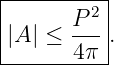
The final exercise goes beyond stationarity and proves the global inequality
for a sufficiently regular simple closed planar curve, using the periodic Wirtinger inequality.
1 Exercises
Exercise 1: set up the graph-form isoperimetric problem
Let a smooth graph y(x) join
with y(x) ≥ 0. Its enclosed area above the x-axis is
and its arc length is
Suppose S[y] = L is prescribed.
- Form an augmented functional whose stationary functions are candidates for maximum
area.
- Derive the Euler–Lagrange equation.
- Show that the stationary graph has constant signed curvature.
Exercise 2: integrate the constant-curvature equation
Continue Exercise 1 and assume the extremal is symmetric about x = 0. Let R > 0 denote the
radius associated with the constant curvature.
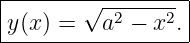
- Show that the upper stationary graph can be written
- Introduce an angle α by
Show that
- Interpret the result geometrically.
Exercise 3: the semicircle special case
For the fixed-chord problem of Exercise 2, suppose
Show that R = a and therefore
Compute the enclosed area.
Exercise 4: Dido’s straight-shoreline problem
A curve of prescribed length L lies above a straight shoreline. Its two endpoints may slide
freely along the shoreline, and together the curve and the shoreline segment enclose an
area.
- Explain why transversality requires the stationary curve to meet the shoreline
orthogonally.
- Combine this endpoint geometry with the constant-curvature result to show that the
stationary curve is a semicircle.
- Find its radius and enclosed area in terms of L.
Exercise 5: closed-curve vector formulation
Let a smooth simple closed curve be represented by
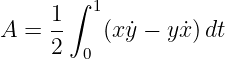
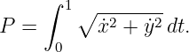
with periodic endpoint conditions. Its oriented area and perimeter are
and
Use a constant multiplier λ to extremize A subject to fixed P.
- Derive the two Euler–Lagrange equations.
- Introduce the unit tangent T and show that its derivative with respect to arc length
has constant magnitude.
- Conclude that every regular stationary closed curve has constant curvature and is
therefore a circle.
Exercise 6: same perimeter, different areas
For a fixed perimeter P, compute the enclosed area of
- a circle;
- a square;
- a regular n-gon.
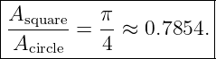
Show that the regular n-gon area tends to the circle area as n →∞. Evaluate the area ratio
Asquare∕Acircle.
Exercise 7: the multiplier as a sensitivity
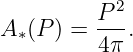
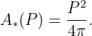
The globally optimal circle of perimeter P has
- Compute dA∗∕dP.
- Express the result in terms of the optimal circle radius R.
- Relate this to the magnitude of the Lagrange multiplier appearing in Exercise 5, noting
that its sign depends on the chosen augmented-functional convention and orientation.
Exercise 8: global proof using the periodic Wirtinger inequality
Let r(s) = (x(s),y(s)) be a regular simple closed curve parametrized by arc length s ∈ [0,P].
Translate the origin so that
Use the following periodic Wirtinger inequality for any mean-zero P-periodic function
f:
Starting from
prove
Explain why equality corresponds to a circle.
2 Solutions
Solution 1: graph formulation and constant curvature
The objective is area,
while the constraint is
Using a constant multiplier λ, define the augmented integrand
The sign of λ is conventional; replacing λ by −λ changes no physics or geometry.
We have
and
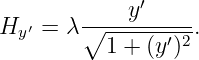
The Euler–Lagrange equation gives
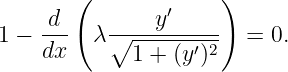
Because λ is constant,
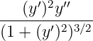
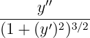
Differentiate explicitly:
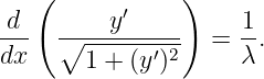
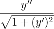
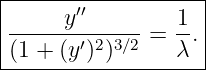
Hence
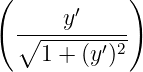
The left-hand side is the signed curvature of the graph. Therefore every smooth stationary graph
has constant signed curvature. A nonzero constant-curvature plane curve is an arc of a
circle.
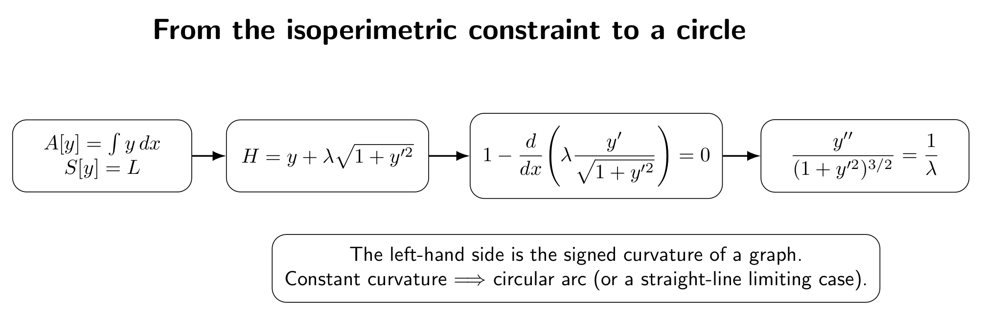
Figure. The constrained area problem becomes an ordinary Euler–Lagrange problem for
the augmented integrand. The resulting differential equation says that the graph curvature
is constant.
This conclusion is a necessary stationarity condition. By itself, it does not yet prove that the circle
is the global maximizer.
Solution 2: integrating to obtain the circular arc
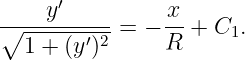
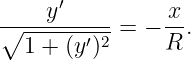
For an upper concave-down arc, it is convenient to write
Integrating once gives
Symmetry about x = 0 implies y′(0) = 0, hence C1 = 0:
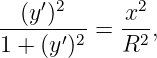
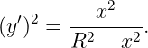
Square and solve for y′:
so
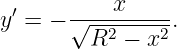
The upper arc has negative slope for x > 0, therefore
Integrating,
The endpoint condition y(a) = 0 gives
hence
This is a circle of radius R whose center lies below the chord.
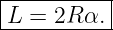
Now define α by
The circular arc subtends the central angle 2α, so its length is
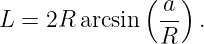
Equivalently,
Thus the prescribed chord and prescribed length together determine the radius of the stationary
circular arc.
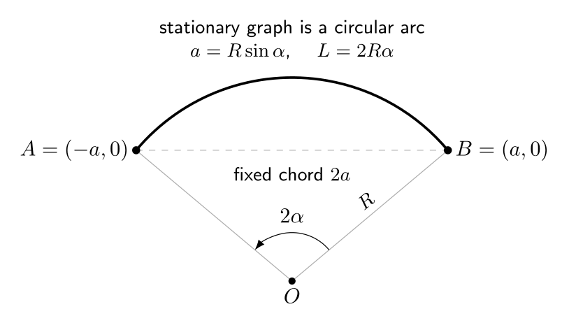
Figure. For a fixed chord 2a, the stationary graph is a circular arc. The chord-radius
relation is a = R sin α and the prescribed arc length is L = 2Rα.
For the graph formulation, the minor-arc family runs from the straight-line limit L → 2a to the
semicircle L = πa.
Solution 3: the semicircle
If
then the circular arc must satisfy
and
The semicircle corresponds to
so
The stationary graph therefore becomes
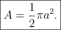
Its area is the area of a semicircle:
Notice the distinction between the semicircle as a stationary solution and the statement that it
gives the largest area among all admissible curves. The latter is a global theorem; Exercise 8
supplies a global argument for the closed-curve version.
Solution 4: Dido’s shoreline problem
The Dido-type problem differs from the fixed-chord problem because the endpoints may slide along
the straight shoreline. Endpoint freedom adds transversality information.
In the graph formulation the shoreline is y = 0. At a sliding endpoint,
while δx is free. The moving-endpoint boundary term from CV05 therefore requires
For
we obtain
| H − y′Hy′ | = y + λ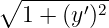 − λ − λ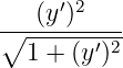 | (51)
|
| = y + 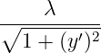 . . | (52) |
At the shoreline y = 0, transversality gives
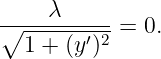
For a nontrivial finite multiplier this requires
Thus the tangent to the stationary arc is vertical at the shoreline: the curve meets the straight
boundary orthogonally.
A constant-curvature arc that meets the same straight line orthogonally at both endpoints must be
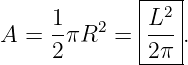
a semicircle. If its radius is R, then its curved-boundary length is
so
The enclosed area is therefore
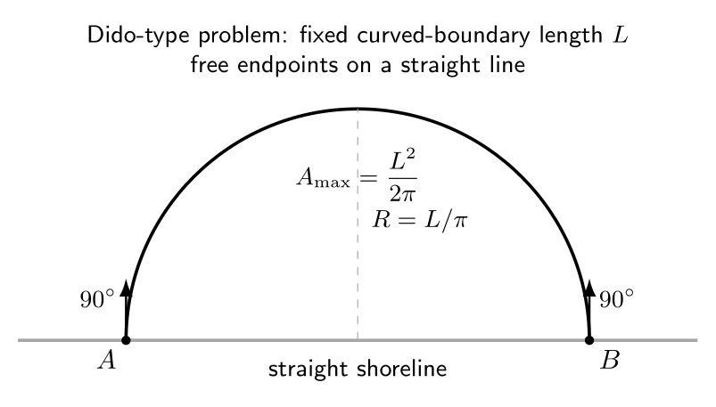
Figure. With a straight shoreline supplied for free, the variational endpoint condition
requires orthogonal contact. Combined with constant curvature, this selects a semicircle.
This is the familiar “Dido problem” version of isoperimetric geometry [2, 6].
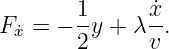
Solution 5: closed curves and the vector Euler–Lagrange equations
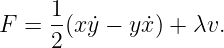
Define
and use the augmented integrand
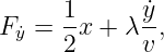
For x,
and
Hence
| 0 | = Fx − Fẋ Fẋ | (62)
|
| =  ẏ − ẏ −![[ ( )]
1- d- ˙x-
− 2y˙+ λ dt v](https://images.physicslibrary.org/cache/objects/1208/make4ht/CalculusOfVariationsTheClassicalIsoperimetricProblemWorkedExamplesAndProofs67x.png) , , | (63) |
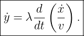
so
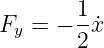
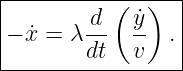
Similarly, for y,
and
which gives
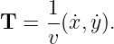
Introduce the unit tangent
Because
we have
The two equations become
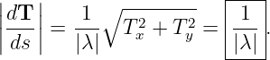
Therefore
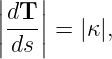
But
so the curvature magnitude is constant. A regular closed plane curve with nonzero constant
curvature is a circle. Thus the vector formulation reaches the same stationary geometry without
privileging a graph coordinate.
This formulation also shows why the multiplier has units of length: its magnitude is the stationary
radius.
Solution 6: comparing equal-perimeter shapes
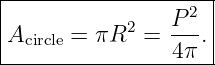
For a circle of perimeter P,
so
Hence
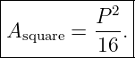
For a square, the side length is P∕4, giving
Therefore
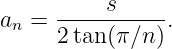
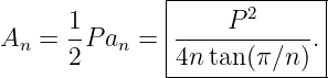
For a regular n-gon of side length s = P∕n, the apothem is
The area is one half perimeter times apothem:
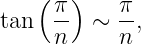
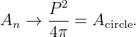
As n →∞,
so
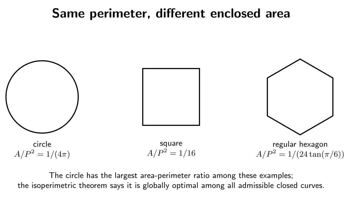
Figure. Simple equal-perimeter comparisons already suggest the isoperimetric theorem.
Regular polygons approach the circle as the number of sides increases.
These comparisons are illustrative, not a proof against all possible curves.
Solution 7: multiplier sensitivity
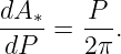
For the globally optimal circle,
Differentiate:
Since
we have
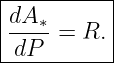
Thus an infinitesimal increase dP in the available perimeter increases the optimal area by
approximately
In Exercise 5, the stationary radius satisfies
The sign depends on whether the augmented functional is written as A + λ(P − P0) or
A − μ(P − P0) and on the orientation of the curve. The magnitude has the sensitivity
interpretation expected from the multiplier discussion in CV09.
Solution 8: the global isoperimetric inequality
Now we prove that the circle is not merely stationary but globally optimal under the stated
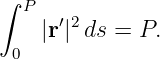
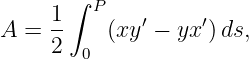
smoothness assumptions. Parametrize the closed curve by arc length s, so
Therefore
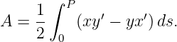
The oriented area is
Introduce the quarter-turn operator
Then
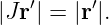
Since J preserves Euclidean length,
Cauchy–Schwarz gives
| |A| | ≤ 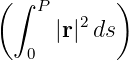 1∕2 1∕2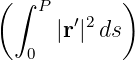 1∕2 1∕2 | (95)
|
| =  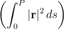 1∕2P1∕2. 1∕2P1∕2. | (96) |
Translate the origin so that both coordinate functions have zero mean. The periodic Wirtinger
inequality gives
and
Add them:
| ∫
0P |r|2 ds | ≤ 2 ∫
0P |r′|2 ds 2 ∫
0P |r′|2 ds | (99)
|
| =  2P 2P | (100)
|
| =  . . | (101) |
Substitute into the Cauchy–Schwarz bound:
| |A| | ≤  1∕2P1∕2 1∕2P1∕2 | (102)
|
| =  . . | (103) |
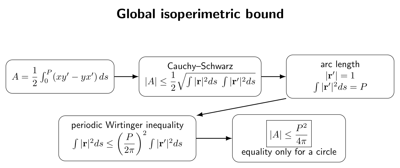
Figure. The global proof combines the area formula, Cauchy–Schwarz, arc-length
parametrization, and the periodic Wirtinger inequality.
To understand equality, both inequalities must be sharp. Equality in the periodic Wirtinger
inequality requires x and y to contain only the first periodic harmonic after centering. Equality in
Cauchy–Schwarz requires the position vector and the quarter-turn of the unit tangent to be
linearly dependent with constant proportionality. Together with unit-speed parametrization, these
conditions reduce to
where
Thus equality is attained by a circle, and the stationary circle found by the multiplier calculation is
indeed the global maximizer. This classical proof strategy and related variants are discussed in
standard treatments of the isoperimetric inequality [4, 6].
3 What the worked examples establish
The examples reveal three logically distinct levels of conclusion.
- Multiplier stationarity: constrained Euler–Lagrange gives constant curvature.
- Endpoint geometry: transversality can select which circular arc is admissible, as in
the Dido semicircle.
- Global optimality: an inequality argument is required to prove that no other
admissible closed curve encloses more area.
It is important not to collapse these three statements into one. Euler–Lagrange supplies a
necessary condition. The isoperimetric inequality supplies the global comparison.
4 Common mistakes
- Calling the circle a maximum immediately after Euler–Lagrange. Constant
curvature identifies stationary candidates; it does not by itself prove global maximality.
- Forgetting the original perimeter constraint. The differential equation gives a
family of circles; the prescribed length fixes the radius or remaining parameter.
- Using a variable multiplier for a single scalar perimeter constraint. The
isoperimetric multiplier is constant.
- Ignoring endpoint freedom in the Dido problem. Sliding endpoints contribute
transversality conditions and force orthogonal contact with the shoreline.
- Confusing the graph formulation with the full closed-curve problem. A single
graph cannot represent every closed curve or every major circular arc.
- Dropping orientation signs. The signed curvature and the multiplier may change
sign if the curve orientation or augmented-functional convention changes; the radius is
positive and corresponds to the magnitude.
- Using the area formula without regularity assumptions. The global proof
assumes a sufficiently regular simple closed curve so that arc-length parametrization
and the line-integral area formula are valid.
5 Bridge to later variational theory
The classical isoperimetric problem anticipates several ideas that recur later in the PhysicsLibrary
CV sequence.
The multiplier behaves like a conjugate sensitivity variable. The closed-curve derivation
is naturally vector-valued, linking directly to CV07. Endpoint orthogonality uses the
transversality ideas of CV05. The constant-curvature result is a geometric first integral in
spirit, linking to CV06. Finally, the global proof requires an inequality rather than only
stationarity, foreshadowing the second-variation and sufficiency theory developed in
CV11–CV13.
References
References
[1] I. M. Gelfand and S. V. Fomin, Calculus of Variations, Dover Publications, 2000.
[2] Hans Sagan, Introduction to the Calculus of Variations, Dover Publications, 1992.
[3] Gilbert Ames Bliss, Lectures on the Calculus of Variations, University of Chicago
Press, 1946.
[4] Richard Courant and David Hilbert, Methods of Mathematical Physics, Volume I,
Wiley-Interscience, 1989 reprint.
[5] Leonhard Euler, Methodus inveniendi lineas curvas maximi minimive proprietate
gaudentes, Lausanne and Geneva, 1744.
[6] Robert Osserman, “The Isoperimetric Inequality,” Bulletin of the American
Mathematical Society, vol. 84, no. 6, pp. 1182–1238, 1978.

![[parent]](https://images.physicslibrary.org/images/uparrow.png)



![∫ a
A [y] = y(x )dx,
−a](https://images.physicslibrary.org/cache/objects/1208/make4ht/CalculusOfVariationsTheClassicalIsoperimetricProblemWorkedExamplesAndProofs3x.png)
![∫ a
S [y ] = ∘1--+-(y′)2dx.
− a](https://images.physicslibrary.org/cache/objects/1208/make4ht/CalculusOfVariationsTheClassicalIsoperimetricProblemWorkedExamplesAndProofs4x.png)








![∫ a
A[y] = −a ydx,](https://images.physicslibrary.org/cache/objects/1208/make4ht/CalculusOfVariationsTheClassicalIsoperimetricProblemWorkedExamplesAndProofs18x.png)
![∫ a
S[y] = ∘1--+-(y′)2-dx = L.
−a](https://images.physicslibrary.org/cache/objects/1208/make4ht/CalculusOfVariationsTheClassicalIsoperimetricProblemWorkedExamplesAndProofs19x.png)