Calculus of Variations: Piecewise-Smooth Extremals and the Weierstrass-Erdmann Corner
Conditions
The classical Euler–Lagrange derivation assumes that the candidate extremal is smooth enough
across the whole interval. Many physical and geometric problems naturally produce a different
situation: the candidate is smooth on separate subintervals but may have an interior point at
which its slope changes. Such a curve is called piecewise smooth, and the interior point is
commonly called a corner.
The central question of this entry is simple to state:
If each smooth segment already satisfies the Euler–Lagrange equation, what
additional conditions must hold where the segments meet?
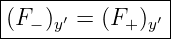
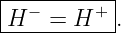
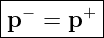
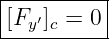
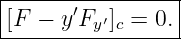
The answer is given by the Weierstrass–Erdmann corner conditions. For a freely movable corner,
two quantities must agree across the corner: the generalized momentum
and the Hamiltonian-like combination
Equivalently, F − y′Fy′ is continuous. These conditions are classical necessary conditions for
broken extremals; see, for example, [1, 2, 3, 4, 5].
1 Piecewise-smooth admissible curves
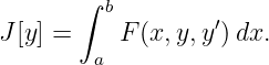
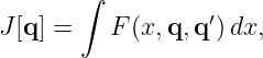
Consider the first-order functional
Suppose a candidate curve is smooth on the two intervals
and is continuous at x = c, but the one-sided slopes may differ:
in general. We write the two pieces as y−(x) and y+(x).
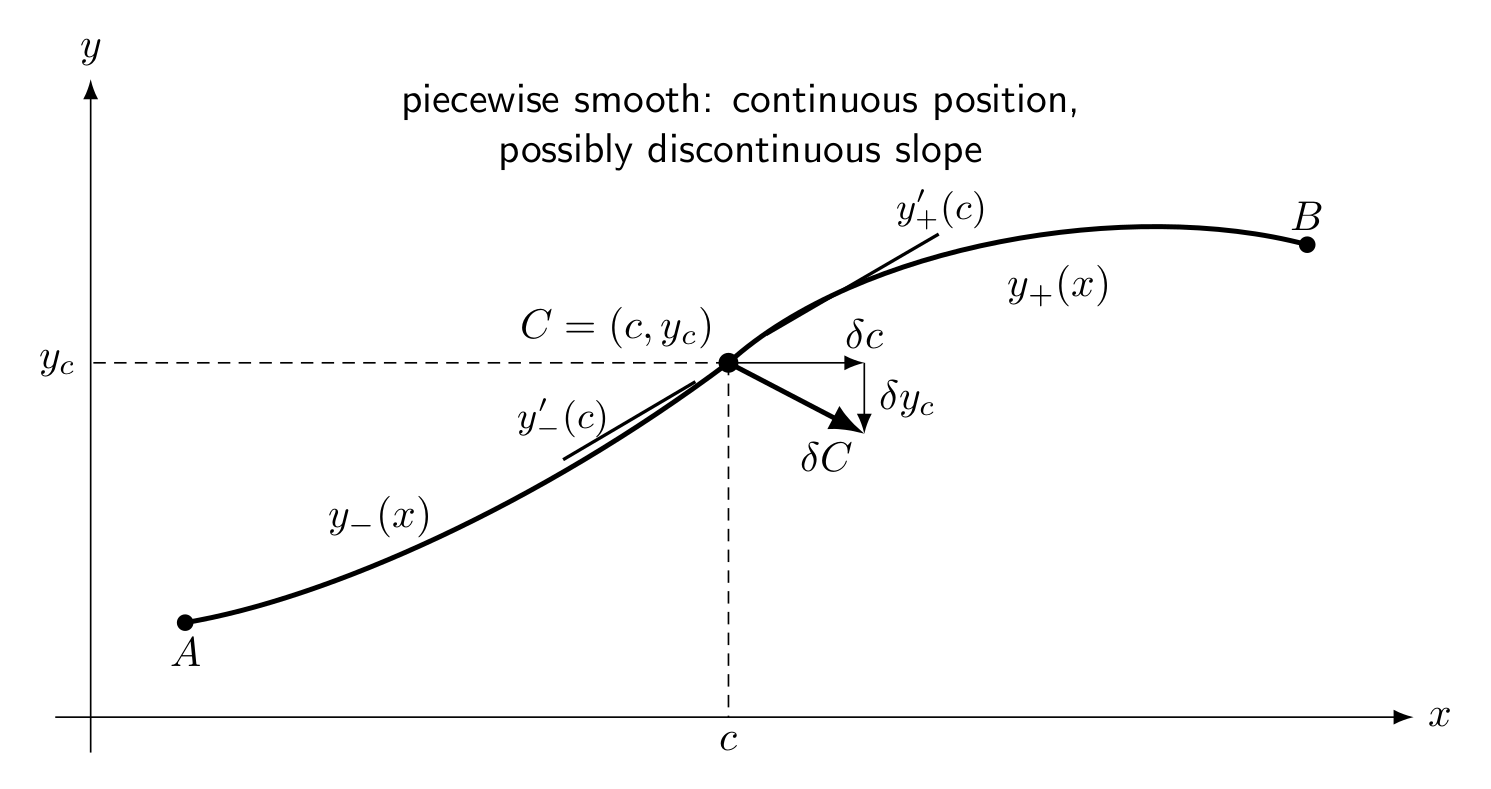
Figure. A piecewise-smooth candidate consists of smooth left and right extremal arcs
joined continuously at an interior corner C = (c,yc). A corner variation can change both
the corner abscissa and the corner ordinate.
The action naturally splits into
The notation F− and F+ allows the two sides to have different constitutive data, as at an optical
or material interface. When the same smooth integrand applies everywhere, simply set
F− = F+ = F.
2 Why Euler–Lagrange is not enough
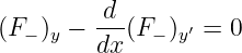
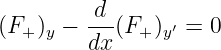
If variations are supported strictly inside (a,c), the usual argument gives
on the left arc. Similarly,
on the right arc.
These equations describe what happens between corners. They do not determine how two extremal
arcs may be joined. That information comes from the boundary terms generated at the internal
splitting point c.
This is the same structural idea encountered in CV05: integration by parts separates interior
Euler–Lagrange information from endpoint information. Here, however, the “endpoint” is shared
by two neighboring arcs.
3 A fixed corner location
Begin with the simpler case in which the corner abscissa c is fixed but its ordinate yc is free to
vary. Since the total curve remains continuous, the two variation fields have the same value at the
corner:
After integrating by parts separately on the two subintervals and imposing Euler–Lagrange on each
interior, the corner contribution is
Therefore
Because the corner ordinate is free, ηc is arbitrary. Hence
Thus even a fixed interface requires continuity of generalized momentum if the crossing point can
slide along that interface.
If both c and yc are prescribed, then there is no free corner variation and no additional matching
condition is produced. The two arcs simply meet at a prescribed pin point.
4 Movable corner geometry
Now allow the corner itself to move. Let
and
The subtle point is that the ordinary variation field η(x) measures change at a fixed value of x,
whereas δyc measures the actual change of the moving corner point. These are not the same
quantity.
For the left arc,
Differentiate with respect to 𝜖 at 𝜖 = 0:
Therefore
The same reasoning on the right gives
These two relations are the bookkeeping step that produces the second corner condition.
5 Variation of an integral with a moving limit
For the left piece,
Differentiating gives the usual first-variation integral plus the moving-upper-limit contribution:
After integration by parts and use of Euler–Lagrange on the left arc, the corner term
becomes
Substitute the moving-corner relation:
| δJ−(c) | = (F
−)y′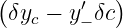 + F−δc | (23)
|
| = (F−)y′δyc +  δc. | (24) |
For the right piece, the corner is a moving lower limit, so the sign reverses:
Adding the two contributions gives
| δJcorner = |  δyc | (26)
|
| +  δc. | (27) |
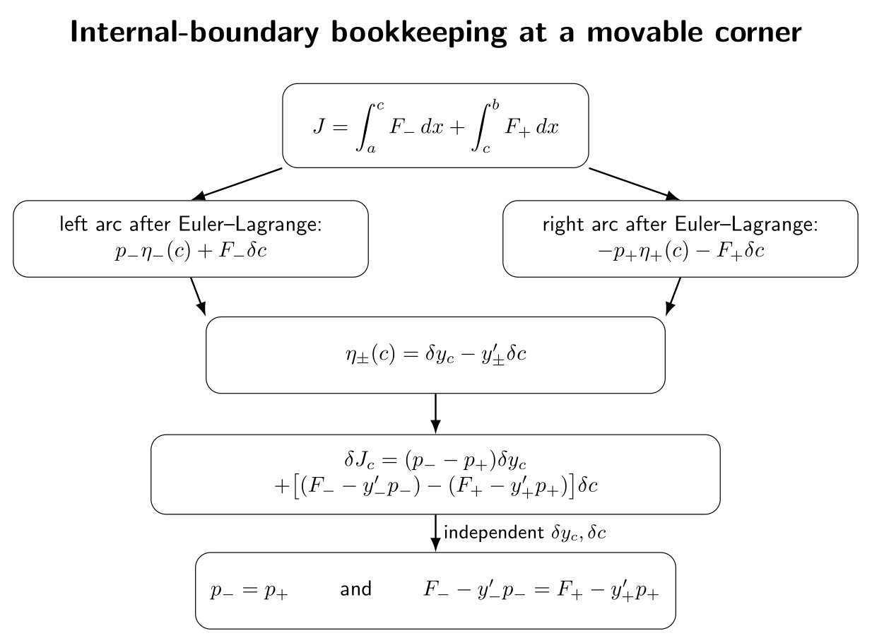
Figure. The corner conditions arise by treating the internal corner as the terminal
endpoint of the left arc and the initial endpoint of the right arc. The endpoint terms
appear with opposite signs.
6 The Weierstrass–Erdmann corner conditions
theorem. Let a piecewise-C1 stationary curve have a freely movable interior corner C = (c,y
c).
Assume each smooth arc satisfies the Euler–Lagrange equation and the one-sided values
needed below exist. If δc and δyc may be varied independently, then the corner must
satisfy
and
These are the Weierstrass–Erdmann corner conditions.
Proof. The preceding derivation gives
where
and
Because δyc and δc are independent, first set δc = 0 and vary δyc to obtain A = 0. Then set
δyc = 0 and vary δc to obtain B = 0. □
It is often convenient to define
and
Then the conditions become simply
and
If the jump notation is
then
7 What the two conditions mean
The first condition comes from moving the corner vertically while holding its abscissa
fixed. It therefore matches the generalized momentum transmitted from one arc to the
other.
The second comes from moving the corner horizontally. It matches the quantity conjugate to shifts
in the independent variable. In mechanics, where the independent variable is time, this is the
Hamiltonian. In autonomous mechanical systems it is the energy.
This is not a coincidence. CV05 already showed that the boundary variation of a first-order
integral may be written schematically as
At an internal corner, the same endpoint expression appears once from the left and once from the
right. Stationarity requires the two endpoint covectors to match.
8 A corner constrained to a prescribed curve
A useful intermediate case occurs when the corner may move, but only along a prescribed
interface
Then the corner displacement satisfies
The two corner variations are no longer independent. Substituting into the general corner term
gives the single transversality condition
| 0 = |  ψ′(c) | (42)
|
| + F−− y−′(F−)y′− F+ + y+′(F+)y′. | (43) |
Thus the fully free Weierstrass–Erdmann pair and the CV05 transversality condition are two
versions of the same boundary-variation geometry.
For a vertical interface x = c, one has δc = 0 while δyc is free, so only generalized momentum
continuity is required.
9 Example: optical refraction and Snell’s law
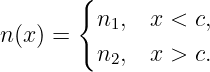
Fermat’s principle makes refraction a particularly transparent corner problem. Suppose Light
travels from a medium of refractive index n1 to a medium of refractive index n2 across the fixed
vertical interface x = c. Apart from a constant factor, the optical travel-time functional
is
with
On each side,
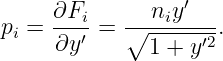
The generalized momentum is
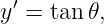
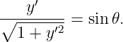
Let 𝜃i be the angle the ray makes with the Normal to the vertical interface. Since
we have
The interface location x = c is fixed, but the crossing height is free. Therefore the fixed-interface
corner condition gives
or
This is Snell’s law.
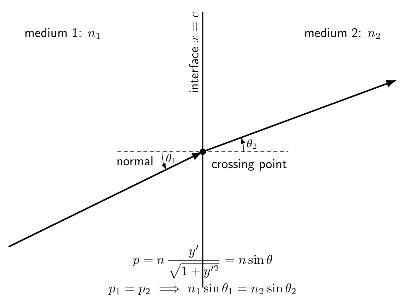
Figure. Refraction is a fixed-interface corner problem. The crossing point may slide along
the interface, so generalized momentum parallel to the interface is continuous. For optical
length this becomes Snell’s law.
The example also explains why a true slope corner is possible: the integrand changes across the
interface because n1≠n2.
10 Example: a quadratic interface problem
Consider
where c is a fixed interface and the crossing ordinate is free. Each side satisfies
so the stationary pieces are straight lines. The corner condition is
Unless k1 = k2, the slope generally changes at the interface. The transmitted quantity is not slope
itself but the generalized momentum p = ky′.
This is mathematically analogous to continuity of flux across many interfaces in diffusion, heat
conduction, elasticity, and wave problems.
11 Why a regular homogeneous integrand usually forbids a genuine corner
Suppose the same smooth integrand F(x,y,y′) applies on both sides of the corner. The first
Weierstrass–Erdmann condition says
If, for fixed (x,y), the map
is one-to-one, then necessarily
A common sufficient local condition is strict convexity in the derivative:
Then Fy′ is strictly increasing as a function of y′, so momentum continuity forces slope
continuity.
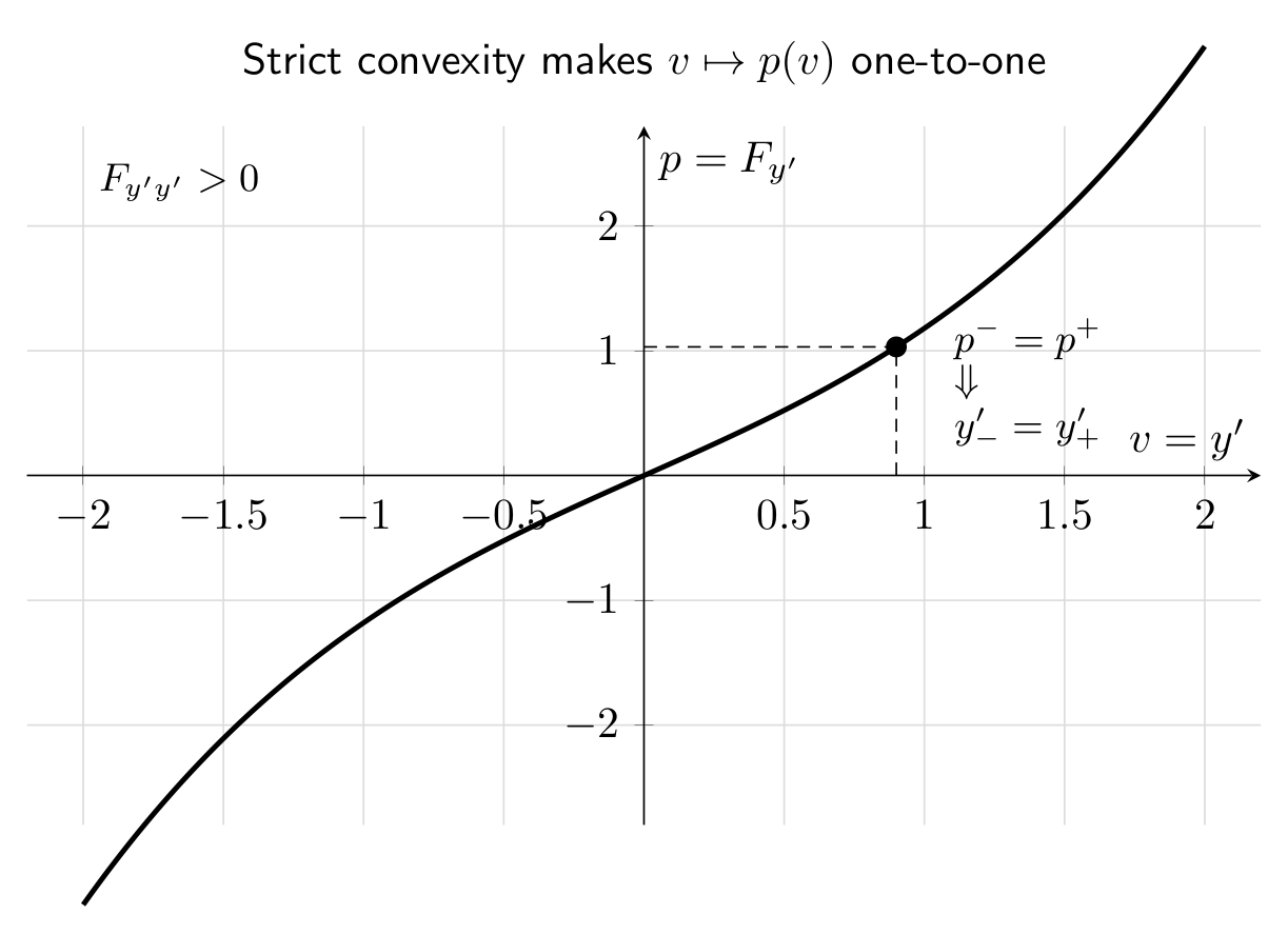
Figure. For a regular strictly convex integrand, the map y′ p = Fy′ is one-to-one. Hence
continuity of p at a corner forces continuity of y′, eliminating a genuine kink when the
same integrand applies on both sides.
This is an important conceptual point: corner conditions do not predict that corners must occur.
Often they prove that a stationary curve cannot have one.
12 Mechanics and a free switching time
Let a trajectory q(t) be governed by one Lagrangian before a switching time tc and another
afterward:
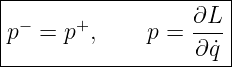
If both the switching state q(tc) and the switching time tc are free, the Weierstrass–Erdmann
conditions become
and
For several coordinates, p becomes a vector and the momentum condition is componentwise.
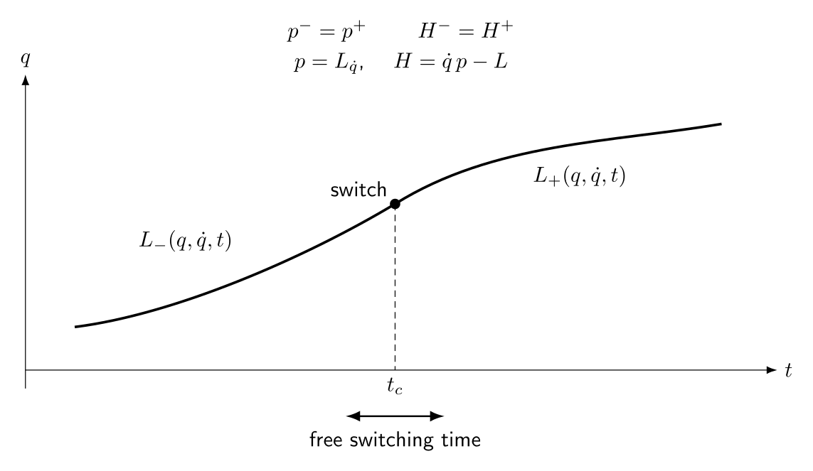
Figure. A free switching time is the mechanical version of a movable corner. Stationarity
matches generalized momentum and Hamiltonian across the switch.
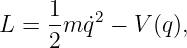
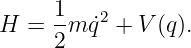
For an ordinary natural mechanical Lagrangian
we have
and
If the same regular Lagrangian applies on both sides and there is no impulse, momentum
continuity forces velocity continuity. Thus a spontaneous velocity kink is incompatible with
stationarity. An actual impulsive force changes the variational model and can produce a
momentum jump.
13 Vector-valued corner conditions
For a vector path q(x) ∈ ℝn and
define the generalized momentum vector
At a freely movable corner the conditions become
and
These are precisely the multi-coordinate forms that recur in mechanics, ray tracing, hybrid
systems, and later optimal-control switching conditions.
14 Several corners
If a broken extremal contains corners
then the first variation splits across all subintervals. Each freely movable interior corner
independently contributes a matching condition. Therefore at every cj,
The logic is local: moving one corner while holding the others fixed isolates its own jump
terms.
15 What if only one corner coordinate is free?
The number of independent corner conditions equals the number of independent corner
displacements.
- If c and yc are both fixed: no corner condition is generated.
- If c is fixed and yc is free: continuity of p.
- If yc is fixed and c is free: continuity of F − y′p, equivalently H.
- If both are free: both Weierstrass–Erdmann conditions.
- If the corner is constrained to a one-dimensional interface: one transversality
combination.
This counting principle is a useful way to avoid imposing too many conditions.
16 Necessary, not sufficient
The Weierstrass–Erdmann conditions are necessary stationarity conditions. They do not by
themselves prove that a broken extremal minimizes the functional.
A candidate may satisfy Euler–Lagrange on every arc and satisfy both corner conditions while still
being a maximum or saddle. Stronger minimum theory requires second-variation conditions,
convexity, the Weierstrass excess function, and related results developed later in the
series.
Likewise, corner conditions do not establish existence. A variational problem may fail to possess a
minimizer even though its formal necessary conditions are well defined.
17 Common mistakes
- Applying Euler–Lagrange separately and stopping. Interior equations do not
contain the corner matching information.
- Assuming η−(c) = η+(c) when the corner moves horizontally. For a movable
corner, η±(c) = δyc − y±′δc.
- Forgetting the moving-limit term F δc. Without it the second
Weierstrass–Erdmann condition is lost.
- Using the same sign for the left and right corner contributions. The corner
is an upper limit for the left integral and a lower limit for the right integral.
- Imposing two conditions when the corner is constrained to an interface.
Only independent corner motions produce independent conditions.
- Assuming a slope kink is always allowed. For a regular strictly convex
homogeneous integrand, momentum continuity typically forces the slope to be
continuous.
- Confusing physical impulses with ordinary corners. An impulse introduces a
momentum jump and therefore changes the stationarity conditions/model.
- Treating the corner conditions as a minimum proof. They are necessary
conditions only.
18 A compact workflow for broken extremals
For a piecewise-smooth candidate, use the following sequence.
- Identify the subintervals and the corner coordinates that are allowed to move.
- Split the functional at every corner.
- Apply Euler–Lagrange separately on each smooth arc.
- Integrate by parts without discarding the internal boundary terms.
- Include moving-limit contributions when a corner abscissa is free.
- Relate fixed-x variations to actual corner displacement through
- Collect coefficients of the independent corner displacements.
- Set those coefficients to zero.
- Interpret the resulting conditions as continuity of generalized momentum and, when the
corner location is free, continuity of the Hamiltonian-like quantity.
- Separately test whether the stationary broken curve is actually minimizing.
19 What CV11 adds
CV10 has completed the main first-order necessary-condition structure for smooth and
piecewise-smooth extremals. The next question is classification: when does a stationary curve
actually behave like a minimum?
CV11 introduces the second variation. The second variation is a quadratic functional in the
perturbation and provides the variational analogue of the Hessian in multivariable calculus. Its
simplest local consequence is the Legendre necessary condition, which constrains the sign of Fy′y′
along a minimizing extremal.
Summary
For a piecewise-smooth extremal with a freely movable corner, Euler–Lagrange must hold
separately on every smooth arc, and the internal boundary terms must vanish under independent
corner motion. The resulting Weierstrass–Erdmann conditions are
and
Equivalently, with
we have
The first condition matches generalized momentum; the second matches the quantity conjugate to
movement of the corner in the independent variable. Fixed interfaces, movable interfaces, optical
refraction, mechanical switching times, and vector trajectories are all variations of this same
internal-boundary principle.
References
[1] I. M. Gelfand and S. V. Fomin, Calculus of Variations, Dover Publications, 2000.
[2] Bruce van Brunt, The Calculus of Variations, Springer, 2004.
[3] Hans Sagan, Introduction to the Calculus of Variations, Dover Publications, 1992.
[4] Robert Weinstock, Calculus of Variations with Applications to Physics and
Engineering, Dover Publications, 1974.
[5] Gilbert Ames Bliss, Lectures on the Calculus of Variations, University of Chicago
Press, 1946.
[6] Cornelius Lanczos, The Variational Principles of Mechanics, Dover Publications,
1986.