EDL00: Home Electrodynamics Laboratory - Roadmap, Bench Setup, Measurement Practice, and
Griffiths Companion
This series develops a practical undergraduate electrodynamics laboratory that can be performed
largely at home with low-voltage bench equipment.
The theoretical companion is David J. Griffiths’ Introduction to Electrodynamics. The laboratory is
independent and unofficial. It does not reproduce textbook problems or replace the derivations in
the text. Instead, it asks a complementary question:
The answer is surprisingly broad.
With one carefully chosen bench, the student can experimentally study
- electric potential and electric fields,
- conductivity and current density,
- capacitance and dielectric response,
- magnetic fields produced by currents,
- ferrites and magnetic materials,
- Faraday induction and mutual inductance,
- RC, RL, and RLC dynamics,
- Maxwell’s displacement-current motivation,
- electromagnetic energy storage and transfer,
- polarization and optical electromagnetic waves,
- propagation and reflection on coaxial transmission lines,
- receiving antennas and near-field coupling,
- and the distinction between near fields and radiation fields.
The program is organized so that the same equipment and components are reused repeatedly. A
resistor, capacitor, ferrite rod, oscilloscope probe, length of coax, or Hall sensor should appear in
several experiments rather than being purchased for only one exercise.
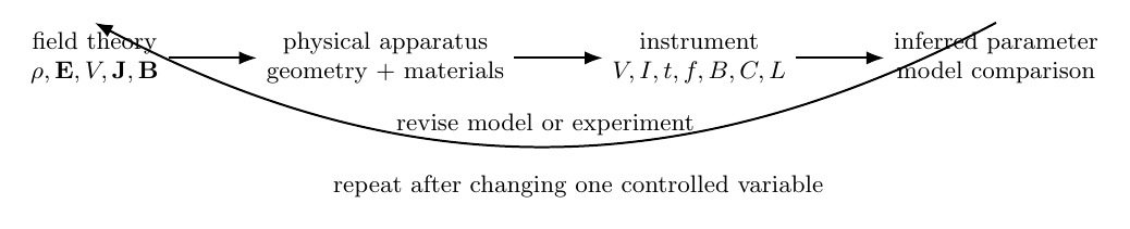
Figure 1. The Electrodynamics Laboratory program repeatedly moves between theoretical fields,
physical apparatus, instrument readings, and inferred parameters. The goal is not merely to
demonstrate an effect, but to measure enough information to compare the apparatus with the
mathematical model.
1 Textbook map
The fifth edition of Griffiths organizes the subject into the following principal chapters:
- Chapter 1 - vector Analysis,
- Chapter 2 - Electrostatics,
- Chapter 3 - Potentials,
- Chapter 4 - Electric Fields in Matter,
- Chapter 5 - magnetostatics,
- Chapter 6 - Magnetic Fields in Matter,
- Chapter 7 - Electrodynamics,
- Chapter 8 - Conservation Laws,
- Chapter 9 - Electromagnetic Waves,
- Chapter 10 - Potentials and Fields,
- Chapter 11 - Radiation,
- Chapter 12 - Electrodynamics and Relativity.
The EDL sequence does not force one experiment onto every chapter. Some topics are much better
suited to controlled home measurements than others. In particular, relativity is better treated
computationally than through a contrived home experiment.
The laboratory sequence is therefore organized around experiments that expose the strongest
measurable connections to the theory.
2 Series philosophy
Each EDL article should follow the same experimental pattern:
For example, a magnetostatics experiment should not stop after showing that a compass needle
moves near a current-carrying wire.
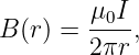
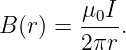
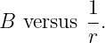
A stronger experiment is to predict
measure B at several values of I and r, plot the data against the predicted scaling variables, and
infer an experimental slope.
Likewise, a capacitance experiment should not stop at identifying a capacitor. It should test
relations such as
by changing area, separation, or dielectric material and comparing the measured trends with the
model.
3 The standard EDL home bench
The program assumes a compact electronics bench rather than a professional research
laboratory.
A good home arrangement has five functional zones:
- Power and source generation,
- time-domain measurement,
- handheld measurement,
- experiment construction,
- data recording and computation.
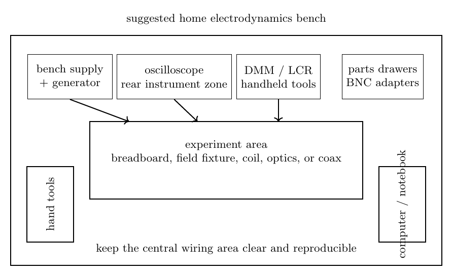
Figure 2. Suggested home-bench layout. The powered instruments remain at the rear, the
experiment stays in the center, and frequently moved probes and leads approach from the sides.
The computer or notebook is kept outside the immediate wiring area.
The bench need not be large. A desk roughly one meter wide is enough for many of the
experiments if storage is organized well.
4 Core instrument 1: digital multimeter
The digital multimeter is the first required instrument.
The EDL program uses it for
- DC voltage,
- DC current,
- resistance,
- continuity,
- diode forward-voltage tests,
- source-resistance experiments,
- coil winding resistance,
- amplifier bias measurements,
- and low-frequency or quasi-static sensor measurements.
A useful minimum feature set is
- at least a 6000-count display,
- DC voltage and current ranges appropriate for low-voltage electronics,
- resistance measurement into the megohm range,
- continuity beeper,
- diode test,
- replaceable fused current ranges,
- and CAT-rated leads from a reputable manufacturer.
Capacitance and frequency modes are convenient but not required. In several EDL labs, we will
deliberately infer capacitance or inductance by another physical method rather than treating a
meter reading as unquestionable truth.
The DMM should usually remain the instrument of choice for static quantities. It should not be
expected to measure small radio-frequency waveforms accurately.
5 Core instrument 2: oscilloscope
The oscilloscope is the most important instrument in the dynamic half of the program.
A good target for a new home bench is
- at least two channels,
- approximately 100 MHz analog bandwidth,
- at least 1 GSa∕s maximum sample rate,
- external trigger input if available,
- math functions including channel subtraction and FFT,
- cursors and automatic measurements,
- USB data export,
- and two switchable 1 × ∕10× passive probes.
A 50 MHz oscilloscope can perform most of the early EDL experiments. A 100 MHz instrument
gives more margin for coaxial-line pulse measurements, fast edges, radio experiments, and later
troubleshooting.
The oscilloscope will be used to measure
- RC and RL transients,
- phase between sinusoidal voltage and current,
- Resonance and bandwidth,
- induced voltages,
- transformer waveforms,
- hysteresis-loop signals,
- pulse reflections on coax,
- photodiode signals,
- and receiving-antenna waveforms.
Probe bandwidth is not the only issue
Every oscilloscope probe loads the circuit under test.
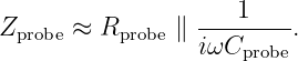
A first model for a passive probe is
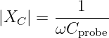
At low frequency the large probe resistance may dominate. As frequency increases, the capacitive
reactance
decreases.
Therefore the act of observing an RLC circuit can shift its resonance or reduce its quality
factor.
This effect is not merely an inconvenience. Several EDL experiments will measure it
deliberately.
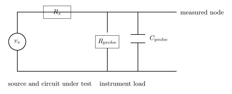
Figure 3. A real measuring instrument becomes part of the circuit. The EDL program treats
instrument loading as measurable physics rather than as an afterthought.
6 Core instrument 3: function generator
The function generator supplies controlled time-varying sources.
A practical target is
- sine, square, and pulse waveforms,
- frequency range from below 1 Hz to at least 10 MHz,
- adjustable amplitude and DC offset,
- burst mode if available,
- sweep capability,
- and AM modulation if available.
A 20–30 MHz two-channel generator is convenient but not mandatory.
The generator will be used for
- RC and RLC excitation,
- inductive coupling,
- transformer measurements,
- displacement-current experiments,
- resonance sweeps,
- transmission-line pulses,
- and controlled RF excitation for antenna experiments.
The generator is not an ideal voltage source
Many bench function generators are designed around a nominal source impedance near
That source resistance matters whenever the load is not much larger than 50 Ω.
The student should learn early to represent the generator by a Thevenin model:
Some generators display amplitude assuming a 50 Ω termination, while others can be switched
between a high-impedance and 50 Ω display convention. EDL01 will make this a measurement
rather than a memorized warning.
7 Core instrument 4: low-voltage bench power supply
The standard EDL supply should be current limited and should remain firmly in the low-voltage
regime.
A practical target is
- adjustable 0–30 V output,
- at least 2–3 A capability,
- adjustable current limit,
- voltage and current displays,
- and output enable control.
A second independently adjustable channel is convenient but not necessary for the core
series.
The most important feature is not maximum voltage. It is a reliable current limit.
For an unfamiliar circuit, begin with a small current limit and increase it only after confirming
expected behavior.
The EDL core does not require direct work with mains voltage or high-voltage capacitor
banks.
8 Strongly recommended instrument: LCR meter
An LCR meter is optional because many EDL labs deliberately infer L and C from dynamic
measurements.
Nevertheless, an inexpensive LCR meter is useful as an independent comparison tool.
It can measure
- capacitance,
- inductance,
- resistance,
- dissipation factor,
- and sometimes equivalent series resistance.
The pedagogically useful sequence is often
rather than the reverse.
9 Strongly recommended sensor: Hall magnetic-field probe
Magnetostatics becomes much more quantitative if the laboratory can measure magnetic flux
density directly.
A useful Hall sensor system should be able to measure fields from approximately tens of microtesla
through at least several tens of millitesla.
Possible implementations include
- a commercial handheld gaussmeter,
- a linear Hall sensor connected to the DMM or oscilloscope,
- a calibrated three-axis magnetometer module,
- or a smartphone magnetometer for coarse experiments.
The preferred EDL approach is a sensor whose raw output voltage can be calibrated against field,
because that preserves the measurement chain.
The Hall system will be used for
- straight-wire magnetic fields,
- circular coils,
- solenoids,
- ferrite-core comparisons,
- and spatial field mapping.
10 Optics kit for electromagnetic-wave labs
Visible Light is an electromagnetic wave and provides several of the cleanest home experiments in
the program.
The required optical kit is modest:
- low-power visible laser module or laser pointer,
- two or three linear polarizing sheets,
- photodiode or phototransistor,
- resistors for a simple detector circuit,
- rotation scale or printed protractor,
- white card or screen,
- and a few transparent dielectric samples.
The polarization laboratory will use these components to test Malus’s law:
The laser should remain low power and should never be aimed toward eyes, reflective jewelry,
mirrors, windows, vehicles, or aircraft.
11 Transmission-line kit
A later laboratory will use coaxial cable as a physically accessible electromagnetic-wave
system.
The useful parts are
- 5–20 m of 50 Ω coaxial cable,
- BNC T adapters,
- BNC barrel adapters,
- 50 Ω feedthrough terminators,
- open and short terminations,
- and BNC-to-clip or BNC-to-header adapters.
Longer cable makes propagation delay easier to resolve on a modest oscilloscope.
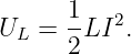
For a line of length ℓ and measured one-way delay td,
The same kit will be reused when studying reflections and impedance matching.
12 The parts drawers
The parts inventory is more important than any single specialized instrument.
A well-organized set of inexpensive passive components makes it possible to change one physical
parameter at a time.
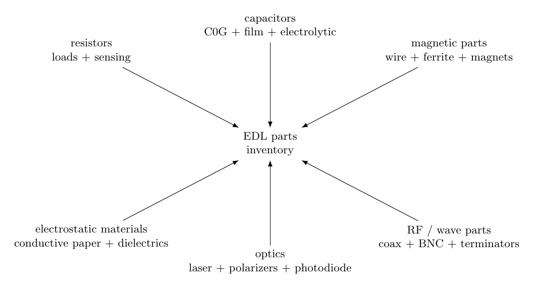
Figure 5. The EDL parts inventory is organized by physical function rather than by one-off
experiment. The same passive components, magnetic parts, optical parts, and RF interconnects
are reused throughout the series.
Resistors
Maintain a 1-percent metal-film assortment with at least the following decade coverage:
Particularly useful values include
Ordinary 1∕4 W resistors are adequate for most labs. Add several 1–5 W power resistors for
low-resistance current and heating experiments.
Capacitors
Maintain several dielectric families because real capacitors are not interchangeable in every
experiment.
For small RF and precision timing values, keep C0G/NP0 ceramic capacitors from roughly
For general timing and filtering, keep film capacitors from approximately
For larger low-frequency time constants and supply decoupling, keep electrolytic capacitors from
approximately
The student should learn that capacitance value alone does not describe a real capacitor.
Equivalent series resistance, leakage, voltage rating, dielectric absorption, tolerance, polarity, and
frequency dependence can matter.
Inductors and magnetic parts
Maintain
- several fixed inductors from roughly 10 μH to 10 mH,
- AWG 26–32 enamel magnet wire,
- ferrite rods,
- ferrite toroids,
- small transformer cores,
- and several small permanent magnets.
Winding coils is part of the curriculum. The student should be able to measure the actual coil
rather than relying only on a nominal value.
Semiconductors
Although Griffiths is not an electronics textbook, a small semiconductor collection is useful for
instrumentation and detector circuits.
Keep
- silicon signal diodes,
- Schottky diodes,
- one or two general-purpose NPN and PNP transistors,
- logic-level MOSFETs,
- a common dual op amp that works from a low-voltage supply,
- photodiodes or phototransistors,
- and linear Hall sensors.
These parts support measurement interfaces without turning the EDL series into a
semiconductor-electronics course.
Conductors and mechanical materials
Useful stock includes
- hookup wire,
- solid-core breadboard wire,
- copper tape,
- aluminum foil,
- brass or copper sheet scraps,
- insulated alligator leads,
- banana leads,
- heat-shrink tubing,
- masking tape,
- card stock,
- acrylic or plastic sheets,
- wood dowels,
- rulers and printed angle scales,
- and nonmagnetic supports.
Many field experiments become easier when the geometry can be reproduced accurately.
13 Breadboards, perfboard, and when not to use them
Solderless breadboards are useful for
- DC circuits,
- low-frequency RC experiments,
- op-amp interfaces,
- Hall-sensor circuits,
- and quick prototyping.
They are less satisfactory for
- high-Q resonant circuits,
- fast pulse edges,
- low-capacitance electrostatic measurements,
- RF circuits,
- and precision transmission-line experiments.
At higher frequency, breadboard contact inductance and inter-row capacitance become part of the
apparatus.
For those experiments use
- small perfboard,
- terminal strips,
- copper-clad board with short point-to-point wiring,
- or a purpose-built fixture with binding posts.
The construction method itself can become an experimental variable.
14 Electrostatics materials
The electrostatics laboratories require several inexpensive non-electronic materials:
- acrylic or PVC rods,
- wool, fur, cotton, and synthetic fabric samples,
- aluminum foil,
- lightweight conductive balls or foil pith balls,
- conductive paper or resistive field-mapping sheets,
- copper tape electrodes,
- paper, acrylic, glass, and plastic dielectric samples,
- and a simple high-input-impedance electrometer interface.
The core series will avoid a high-voltage bench supply. Triboelectric charging, electrostatic
induction, conductive-paper mapping, and capacitor measurements are sufficient to expose much of
the relevant physics safely.
15 Mechanical measurement tools
Electrodynamics experiments depend strongly on geometry.
The home bench should therefore include
- metric ruler,
- digital calipers,
- printed protractors,
- measuring tape,
- small digital scale,
- thermometer,
- and clamps or third-hand fixtures.
These tools often contribute more to measurement quality than a more expensive oscilloscope.
16 Computer and software
The computer is part of the laboratory, but it should not hide the experiment.
The standard workflow should support
Suitable tools include Python with NumPy, SciPy, pandas, and Matplotlib; GNU Octave;
MATLAB; or Julia.
PhysicsLibrary computational companions can provide scripts in more than one language when
doing so helps the learner compare methods rather than software syntax.
A typical laboratory result should include both the raw measurements and the processing script
used to create the final plot.
17 Companion lab files in the PhysicsLibrary filebox
EDL00 includes two reusable companion files intended to live in this article’s PhysicsLibrary
filebox. Upload the files using the exact filenames shown below. Once they are attached to the
EDL00 object, the links in this section provide direct downloads from the article.
The bench checklist is intended to be printed or kept beside the laboratory workspace. It records
the minimum instrument, grounding, current-limiting, and setup checks that should be completed
before beginning a new EDL experiment.
The parts inventory is a machine-readable CSV that can be edited as the home laboratory
grows. It separates core components from optional additions so that later EDL articles
can reference the same standard stock rather than repeating a new shopping list each
time.
Keep these filenames unchanged when uploading them to the filebox:
- EDL00_BENCH_CHECKLIST.txt
- EDL00_core_parts_inventory.csv
18 The standard measurement chain
Every measurement should be viewed as a chain:
| physical quantity | →sensor or coupling element→instrument input | |
|
| →displayed number→inferred quantity. | | |
For example, in a magnetic-field measurement,
Each arrow can introduce uncertainty, loading, calibration error, offset, noise, or bandwidth
limitation.
The EDL program should repeatedly ask:
- What is the instrument actually measuring?
- What physical model converts that reading to the desired quantity?
- What loading did the measurement add?
- What range of frequencies can the instrument follow?
- What systematic errors remain even if the reading is repeatable?
19 Oscilloscope ground and common-reference rules
Many benchtop oscilloscopes connect the BNC shells and probe ground clips to protective
earth.
That means the two probe grounds on an ordinary grounded scope are not independent
nodes.
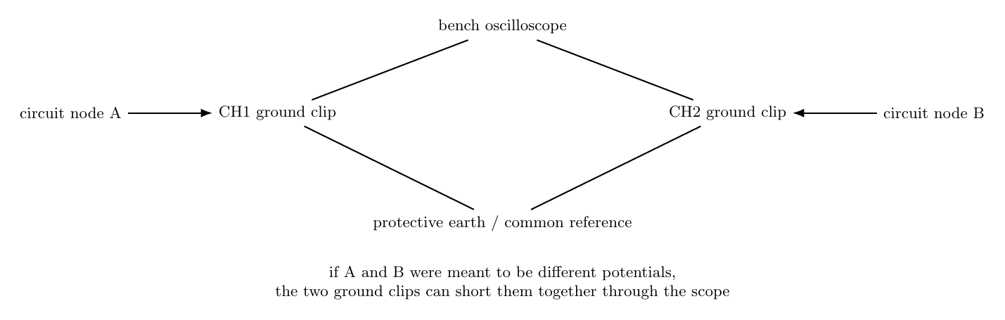
Figure 4. Ordinary grounded oscilloscope channels commonly share the same earth-referenced
ground. Connecting two probe ground clips to two different circuit potentials can therefore short
those nodes together through the oscilloscope.
The standard EDL rule is:
- choose one circuit node as the oscilloscope reference,
- connect all ordinary probe grounds only to that reference,
- never float a mains-powered oscilloscope by defeating protective earth,
- use differential or isolated probes when a true floating measurement is required,
- and do not connect the EDL bench directly to mains wiring.
This rule is both a safety requirement and a measurement-quality requirement.
20 Low-voltage safety boundary
The core EDL series is intentionally designed around low-voltage experiments.
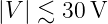
The Normal bench boundary is
from current-limited laboratory supplies, batteries, or signal generators.
The series does not require
- exposed mains voltage,
- microwave-oven transformers,
- flyback-transformer experiments,
- charged high-voltage capacitor banks,
- Tesla coils,
- or high-power RF transmitters.
Electrostatics demonstrations can produce high potentials with very small stored energy, but even
then the apparatus should be kept away from sensitive electronics, combustible vapors, and people
with implanted medical devices.
Laser work should remain low power and use a controlled beam path below eye level.
Strong permanent magnets should be kept away from magnetic storage, watches, pacemakers, and
pinch-sensitive body parts.
21 Current limiting as a standard practice
Before applying power to an unfamiliar circuit:
- set the supply voltage to zero or disable the output,
- choose a conservative current limit,
- inspect the wiring,
- connect the DMM or scope if appropriate,
- enable the supply,
- raise voltage while watching current,
- stop immediately if current differs substantially from prediction.
This procedure is more valuable than memorizing a list of component failure modes.
22 Data notebooks and file naming
Every experiment should produce enough information to be repeated.
At minimum record
- date,
- experiment identifier,
- circuit or geometry sketch,
- component values and measured tolerances,
- instrument models and settings,
- probe attenuation,
- source amplitude and frequency,
- environmental details when relevant,
- raw data,
- observations,
- and any deviations from the article procedure.
A useful file structure is
EDL06/
  raw/
  photos/
  analysis/
  plots/
  notes/
Do not overwrite raw data after analysis. Derived quantities should be reproducible from the raw
measurements.
23 Uncertainty and repeatability
The home laboratory should not pretend that every displayed digit is physically meaningful.
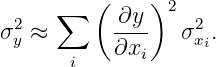
Suppose a quantity y depends on measured variables x1,x2,…:
For small independent uncertainties, a first-order estimate is
The core EDL articles do not need a full metrology treatment, but each should identify the
dominant uncertainties.
Examples include
- electrode spacing in a capacitor experiment,
- Hall-sensor offset in a magnetostatics experiment,
- oscilloscope probe capacitance in a resonator experiment,
- cable length and trigger threshold in a propagation-delay experiment,
- polarizer angle in a Malus-law experiment,
- and background RF in an antenna experiment.
Repeated measurements should be used to distinguish random scatter from systematic
disagreement.
24 The standard EDL workflow
Every major experiment should contain the following sections.
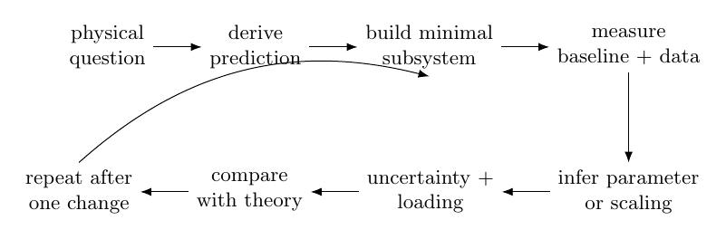
Figure 6. Standard EDL workflow. A laboratory result is complete only after the prediction and
measurement have been compared and the limitations of the measurement have been identified.
- State the physical question.
- Derive the prediction to be tested.
- Identify the independent and dependent variables.
- Build the smallest subsystem capable of testing the prediction.
- Measure component values before assembly when practical.
- Perform a control or baseline measurement.
- Acquire the main data set.
- Change one physical parameter and repeat.
- Plot the quantity that should reveal the theoretical scaling most directly.
- Infer one or more physical parameters from the data.
- Estimate uncertainty and identify instrument loading.
- Compare experiment with theory.
- Explain disagreement before changing the model or discarding data.
25 EDL01 - Practical Electricity and Measurement for Electrodynamics
This article supplies practical electrical knowledge that Griffiths reasonably assumes but a home
laboratory must make explicit.
Measurements include
- Ohm’s law using independent voltage and current measurements,
- loaded voltage dividers,
- DMM input resistance,
- function-generator source resistance,
- oscilloscope probe loading,
- RC charging and discharging,
- component tolerance,
- and common-ground oscilloscope behavior.
A central result will be the experimentally inferred Thevenin model
This article becomes the practical prerequisite for the remaining series.
26 EDL02 - Electrostatics, Charge, Induction, and an Electrometer
Griffiths connection: Chapter 2.
The laboratory uses triboelectric charging and a high-input-impedance detector to study
- sign of charge,
- attraction and repulsion,
- charging by contact,
- charging by induction,
- Conductor shielding,
- and qualitative field behavior.
The objective is not precision measurement of the elementary charge. It is controlled observation of
electrostatic response and conductor boundary behavior without requiring a high-voltage
supply.
27 EDL03 - Potential Mapping, Electric Fields, and Laplace’s Equation
Griffiths connection: Chapters 2 and 3.
Using conductive paper or a resistive sheet, measure
on a regular grid.
Reconstruct the electric field numerically:
Then calculate a finite-difference approximation to
Away from electrodes and sources, the measurements should approximate
This connects boundary-value mathematics to a directly measured potential map.
28 EDL04 - Capacitance, Dielectrics, and Electric Fields in Matter
Griffiths connection: Chapters 3 and 4.
Construct a parallel-plate capacitor with adjustable geometry.
Measure
Compare with
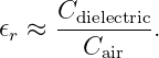
Insert paper, plastic, acrylic, or glass and estimate an effective relative permittivity
from
Fringing and imperfect geometry become part of the uncertainty analysis.
29 EDL05 - Current Density, Conductivity, and Real Conductors
This is a practical bridge into magnetostatics.
Measure the resistance of conductors as a function of
- length,
- cross-sectional area,
- and material where practical.
Test
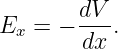
Measure voltage along a long resistive wire and infer the local electric field from
Using
connect the experiment to
30 EDL06 - Biot-Savart Law and Ampere’s Law
Griffiths connection: Chapter 5.
Use a Hall sensor to measure magnetic fields from
- a long straight wire,
- a circular loop,
- and a finite solenoid.
For the straight wire, test
The principal plots are
and
The solenoid experiment will map the departure of a finite coil from the ideal infinite-solenoid
approximation.
31 EDL07 - Magnetic Materials, Ferrites, Inductance, and Hysteresis
Griffiths connection: Chapter 6.
Compare the same coil with
- air core,
- ferrite core,
- and other magnetic cores where appropriate.
Infer inductance from resonance and compare the resulting values.
A more advanced portion uses drive and sense windings to construct a qualitative hysteresis
loop.
The laboratory connects
with actual magnetic materials.
32 EDL08 - Faraday’s Law, Lenz’s Law, Mutual Inductance, and Transformers
Griffiths connection: Chapter 7.
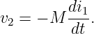
Move a permanent magnet through a coil and measure
Reverse the magnet and reverse the motion to test the sign implied by Lenz’s law.
Then use two stationary coils and measure
Infer M versus
- coil separation,
- orientation,
- frequency,
- and ferrite-core position.
Finish by measuring transformer voltage ratio and loading.
33 EDL09 - Capacitor Current, RLC Dynamics, and Maxwell’s Displacement Current
Griffiths connection: Chapter 7.
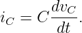
Measure capacitor current using a known series resistor.
Verify
For sinusoidal excitation, observe the phase relation between capacitor voltage and
current.
Then connect the circuit description to the Ampere-Maxwell law: conduction current exists in the
wire, while the changing electric flux through the capacitor gap supplies the displacement-current
term.
The same article should develop measured RC, RL, and RLC transients as preparation for
field-energy accounting.
34 EDL10 - Electromagnetic Energy and the Poynting View
Griffiths connection: Chapter 8.
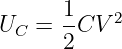
Measure energy stored in
and
Use an underdamped RLC circuit to observe exchange between electric and magnetic energy while
resistance removes energy from the oscillation.
Then interpret the circuit in terms of field energy density and the Poynting vector.
This article should emphasize that electromagnetic energy is carried and stored by fields, not
simply transported as an undefined substance inside the copper wire.
35 EDL11 - Electromagnetic Waves and Polarization
Griffiths connection: Chapter 9.
Use visible light as a convenient electromagnetic wave.
Measure transmitted photodiode signal through two linear polarizers and test
Then add a third polarizer between crossed polarizers and observe the restoration of nonzero
transmission.
Optional extensions include Brewster-angle reflection and polarization by reflection.
36 EDL12 - Propagation and Reflection on Coaxial Transmission Lines
Griffiths connection: Chapter 9, with circuit-level preparation for distributed electromagnetic
systems.
Inject a fast edge or pulse into a long 50 Ω coaxial line.
Measure propagation delay and infer
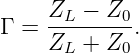
Compare open, shorted, and matched terminations through the reflection coefficient
This is the bridge from lumped-element circuits to finite-speed wave propagation.
37 EDL13 - Antennas, Near Fields, and Radiation
Griffiths connection: Chapters 10 and 11.
Reuse apparatus from the Radio Build Lab.
Excite a small loop or dipole at low power and measure received signal versus
- orientation,
- separation,
- polarization,
- and frequency.
The experiment should emphasize that close to the source the field is not yet a simple pure
radiation field proportional to 1∕r.
The student should compare near-field coupling measurements with the asymptotic radiation-field
picture developed theoretically.
38 EDL14 - Relativistic Electrodynamics as a Computational Laboratory
Griffiths connection: Chapter 12.
No artificial home experiment is required merely to preserve numbering symmetry.
Instead, use computational exercises to transform measured or idealized electric and magnetic
fields between inertial frames.
The objective is to connect experimentally familiar quantities
with their relativistic transformation structure.
This article can also revisit the field of a current-carrying wire from different frames and
demonstrate how electric and magnetic descriptions mix under Lorentz transformation.
39 Series roadmap
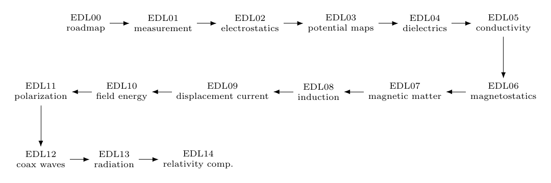
Figure 7. Core EDL sequence. Practical measurement skills come first, then electrostatics,
magnetostatics, induction, energy, waves, radiation, and finally the computational relativity
bridge.
The core sequence is
- EDL00 - roadmap, bench setup, safety, and measurement practice,
- EDL01 - practical electricity and measurement,
- EDL02 - electrostatics and charge,
- EDL03 - potential mapping and Laplace’s equation,
- EDL04 - capacitance and dielectrics,
- EDL05 - current density and conductivity,
- EDL06 - Biot-Savart and Ampere’s law,
- EDL07 - magnetic materials and hysteresis,
- EDL08 - Faraday induction and transformers,
- EDL09 - RLC dynamics and displacement current,
- EDL10 - electromagnetic energy and Poynting flow,
- EDL11 - electromagnetic-wave polarization,
- EDL12 - transmission-line propagation and reflection,
- EDL13 - antennas, near fields, and radiation,
- EDL14 - relativistic electrodynamics computational laboratory.
40 Relationship to the existing PhysicsLibrary EM series
The EDL articles should not rederive material already available in the PhysicsLibrary EM
sequence unless a derivation is needed locally to understand a measurement.
The existing EM series can supply theoretical background for
- Gauss’s Law and electrostatic fields,
- potentials and boundary conditions,
- Ampere’s law,
- Faraday induction,
- the Ampere-Maxwell law,
- Maxwell’s equations,
- electromagnetic waves,
- Poynting energy flow,
- radiation,
- and antenna concepts.
EDL therefore serves as the experimental companion to both Griffiths and the existing PL theory
sequence.
41 Relationship to the Radio Build Lab
The Radio Build Lab and EDL series should deliberately share apparatus.
The following Radio Build Lab hardware transfers directly into EDL:
- ferrite rods,
- magnet wire,
- coupling loops,
- C0G capacitors,
- resistor assortments,
- oscilloscope and probes,
- function generator,
- DMM,
- bench supply,
- BNC adapters,
- and later SDR equipment.
The same ferrite-loop experiment can therefore be interpreted first as a radio-receiver subsystem
and later as a controlled Faraday-law and mutual-inductance experiment.
This reuse is intentional.
42 Buying the bench in stages
The complete laboratory need not be purchased at once.
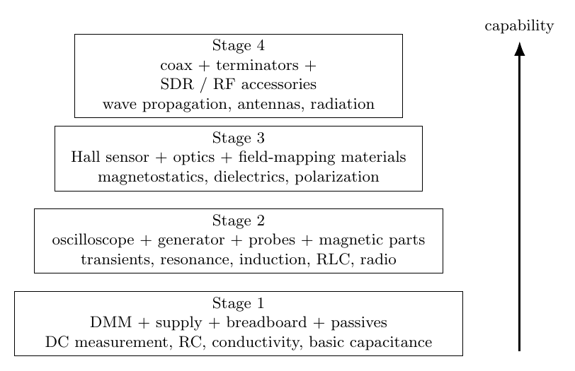
Figure 8. Capability ladder for building the home EDL bench. The core instruments unlock most
early labs; magnetic, optical, transmission-line, and RF accessories are added only when their
part of the curriculum is reached.
Stage 1 - start here
Purchase or assemble
- DMM,
- current-limited low-voltage bench supply,
- breadboards and leads,
- resistor and capacitor assortments,
- hookup wire,
- basic hand tools,
- notebook or computer data workflow.
This supports EDL01 and much of EDL04 and EDL05.
Stage 2 - dynamic measurements
Add
- oscilloscope,
- two 10× probes,
- function generator,
- BNC adapters,
- magnet wire,
- fixed inductors,
- ferrite parts.
This opens most of EDL06 through EDL10 and the Radio Build Lab.
Stage 3 - field sensors and optics
Add
- Hall sensor or gaussmeter,
- low-power laser,
- polarizing sheets,
- photodiode,
- conductive field-mapping paper,
- permanent magnets,
- dielectric samples.
This completes most electrostatic, magnetic, and optical field measurements.
Stage 4 - wave propagation and RF
Add
- long 50 Ω coaxial cable,
- BNC T adapters,
- feedthrough terminators,
- SDR receiver if desired,
- additional RF adapters,
- and low-parasitic construction materials.
This supports the transmission-line, antenna, radiation, and SDR extensions.
43 A recommended home-lab inventory
A mature EDL bench should eventually contain approximately the following categories.
Instrumentation
- 2- or 4-channel digital oscilloscope,
- two or more 10× passive probes,
- function/arbitrary waveform generator,
- digital multimeter,
- current-limited bench supply,
- optional LCR meter,
- optional SDR receiver,
- Hall magnetic-field sensor,
- photodiode detector.
Passive components
- 1-percent resistor assortment,
- C0G/NP0 ceramic capacitor assortment,
- film capacitor assortment,
- electrolytic capacitor assortment,
- fixed inductors,
- potentiometers,
- 50 Ω terminators and loads.
Magnetic and RF materials
- enamel magnet wire,
- ferrite rods,
- ferrite toroids,
- small magnets,
- coax cable,
- BNC adapters,
- copper tape,
- short RF hookup wire.
Electrostatic and dielectric materials
- conductive paper,
- foil electrodes,
- acrylic and PVC rods,
- fabric charging materials,
- dielectric sheets,
- insulating supports.
Optical materials
- low-power laser,
- linear polarizers,
- photodiode or light sensor,
- white screen,
- rotation fixture,
- glass and acrylic samples.
Construction and measurement accessories
- solderless breadboards,
- perfboard and terminal strips,
- soldering iron and solder,
- side cutters and wire strippers,
- tweezers and small pliers,
- banana leads,
- alligator leads,
- probe hooks,
- digital calipers,
- ruler and measuring tape,
- clamps and third-hand fixtures,
- heat-shrink tubing,
- labels and storage drawers.
44 Parts organization
A laboratory becomes dramatically easier to use when parts can be found without searching
through mixed bags.
Organize small drawers or labeled containers by physical family:
- resistors by decade,
- small precision capacitors,
- film capacitors,
- electrolytics,
- inductors and ferrites,
- diodes and transistors,
- sensors,
- RF adapters,
- optical parts,
- mechanical fixtures.
Keep a small “measured parts” tray for components whose actual values have already been
characterized.
That makes repeated experiments much faster.
45 Minimum versus ideal bench
The EDL program should remain accessible.
A minimum bench can use
- one DMM,
- one two-channel oscilloscope,
- one function generator,
- one low-voltage supply,
- inexpensive discrete components,
- homemade sensors where practical.
An idealized advanced bench might add
- four-channel oscilloscope,
- differential probe,
- LCR meter,
- calibrated gaussmeter,
- precision source meter,
- network analyzer or NanoVNA,
- SDR,
- electronic load,
- and data-acquisition hardware.
None of these advanced instruments should be required unless the experiment truly benefits from
them.
The EDL design principle is to infer as much physics as possible from ordinary instruments
first.
46 Completion criterion for the EDL program
The core program is complete when the student can move confidently among three descriptions of
the same physical system:
Examples include
- converting a measured potential map into an electric field,
- converting Hall voltage into magnetic flux density,
- converting induced voltage into mutual inductance,
- converting capacitor current into changing electric flux,
- converting pulse delay into wave velocity,
- converting polarization angle into transmitted intensity,
- and connecting received RF voltage to antenna orientation and field structure.
The objective is not to reproduce a commercial instructional laboratory at home.
The objective is to make undergraduate electrodynamics experimentally tangible enough that the
mathematical objects in the textbook correspond to quantities the student has personally
generated, measured, plotted, and questioned.
47 Summary
The EDL series uses a common home bench to follow the progression
| charge and potential | →electric fields→currents→magnetic fields | |
|
| →induction→field energy→waves→radiation. | | |
The bench grows in stages rather than all at once.
The essential equipment is
- DMM,
- oscilloscope,
- function generator,
- current-limited low-voltage power supply,
- passive component assortments,
- magnet wire and ferrites,
- basic mechanical measurement tools,
- and a computer for plotting and numerical analysis.
The next article, EDL01, establishes the electrical and measurement skills that the rest of the
experimental program will assume.
References
[1] D. J. Griffiths, Introduction to Electrodynamics, 5th ed., Cambridge University Press,
2023.
[2] Cambridge University Press, Introduction to Electrodynamics, Fifth Edition: Contents
and Book Information, 2023.
[3] Tektronix, How to Minimize Probe Loading with Low Capacitance Probes.
[4] P. Horowitz and W. Hill, The Art of Electronics, 3rd ed., Cambridge University Press,
2015.
[5] ARRL, The ARRL Handbook for Radio Communications.
[6] OpenStax, University Physics, Volume 2, Rice University.