Separation of Variables, Membranes, and Two-Dimensional Normal Modes

(Topic)

Separation of Variables, Membranes, and Two-Dimensional Normal Modes

M06-16 introduced the two-dimensional wave equation. We now apply it to a stretched membrane and use separation of variables to derive its normal modes.

For a uniform membrane under equal tension in all in-plane directions,

|---------------------| σutt = 𝒯 (uxx + uyy), | -----------------------

(1)

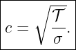
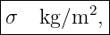
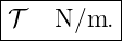
where u(x,y,t) is transverse displacement, σ is surface mass density, and 𝒯 is membrane tension per unit length.

Therefore

|----∘-----| | 𝒯 | |c = --.| --------σ--

(2)

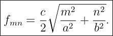
For a rectangular membrane with side lengths a and b fixed on all four edges, the normal-mode shapes are

|-----------------------------------| | (m-πx-) ( nπy-) | Φmn (x,y ) = sin a sin b , | -------------------------------------

(3)

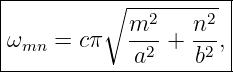
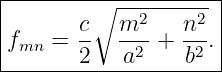
and the frequencies are

|--------∘---------------------------------| |f = c- m2-+ n2, m, n = 1,2,3, ...| --mn----2---a2----b2-----------------------|

(4)

This article derives these results and then develops nodal lines, degeneracy, orthogonality, and modal expansion of arbitrary initial conditions.

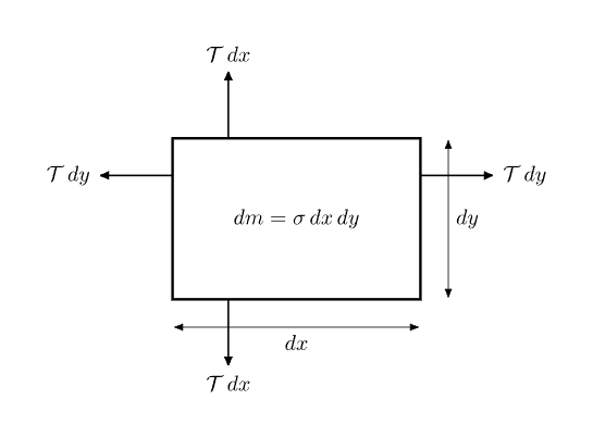
Figure 1. A small rectangular membrane element. Uniform tension per unit length acts along the edges, and small differences in slope produce the transverse restoring force.

1 Membrane parameters

A string uses linear mass density

μ kg ∕m,

(5)

and tension

T N.

(6)

A membrane instead uses surface mass density

|----------| | 2 | σ---kg∕m--,-

(7)

and tension per unit length

|----------| |𝒯 N ∕m. | -----------

(8)

The dimensions of

𝒯 ∕σ

(9)

are

m2 ∕s2,

(10)

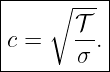
so its square root has dimensions of speed.

2 Derivation of the membrane wave equation

Consider an element of dimensions

dx by dy.

(11)

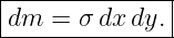
Its mass is

|--------------| -dm--=-σ-dxdy.-|

(12)

Assume uniform isotropic tension, small transverse displacement, small slopes, and negligible bending stiffness.

For the pair of edges Normal to the x direction, the change in transverse tension component is

dFz,x = 𝒯 dy [ux (x + dx, y,t) − ux(x,y,t)].

(13)

Using

u (x + dx,y,t) − u (x,y,t) ≈ u dx, x x xx

(14)

we obtain

|--------------------| |dF = 𝒯 u dx dy. | ----z,x------xx-------

(15)

The pair of edges normal to the y direction similarly contributes

|-------------------| dFz,y-=-𝒯-uyy dx-dy.-

(16)

Thus

dFz = 𝒯 (uxx + uyy) dxdy.

(17)

Newton’s second law gives

σdx dy utt = 𝒯 (uxx + uyy )dx dy.

(18)

Canceling the area gives

|--------------------| -utt =-c2-(uxx-+-uyy-),

(19)

where

|--------| |c2 = 𝒯-.| ------σ---

(20)

3 Separation of variables

Seek a normal-mode solution in product form:

|--------------------------| |u(x,y,t) = X (x)Y (y)Q(t).| ----------------------------

(21)

This is a mode ansatz. A general motion need not be one product; it will be built later as a superposition of many such modes.

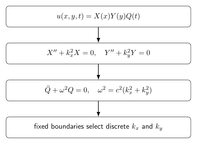
Figure 2. Separation of variables factors a membrane mode into independent x, y, and time factors. The boundaries quantize the spatial factors, and each allowed pair fixes one modal frequency.

Substitution into

2 utt = c (uxx + uyy)

(22)

gives

¨ 2 ′′ ′′ XY Q = c (X YQ + XY Q) .

(23)

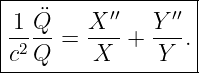
Divide by

2 c XY Q :

(24)

|------------------| | ¨ ′′ ′′ | |1-Q- = X--+ Y--.| -c2Q-----X-----Y---

(25)

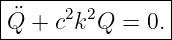
The left side depends only on time while the right side depends only on space, so both must equal a constant. For oscillatory solutions choose

2 − k .

(26)

Then

|----------------| -Q¨+--c2k2Q--=-0.-|

(27)

Thus

|------------------------------------------| |Q (t) = A cos(ωt ) + B sin(ωt), ω = ck. | -------------------------------------------

(28)

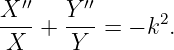
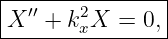
The spatial equation is

′′ ′′ X--- Y-- 2 X + Y = − k .

(29)

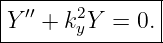
Separate again by writing

--------------- |2 2 2 | k--=-k-x +-ky,-

(30)

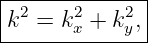
with

|---------------| X ′′ + k2xX = 0, | -----------------

(31)

and

|--------------| |Y′′ + k2yY = 0.| ----------------

(32)

4 Fixed rectangular membrane

Let the membrane occupy

0 ≤ x ≤ a, 0 ≤ y ≤ b.

(33)

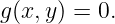
All four edges are fixed:

|------------------------| -u(0,y,t) =-u(a,y,t)-=-0,-

(34)

and

|------------------------| -u(x,0,t) =-u(x,b,t)-=-0.-

(35)

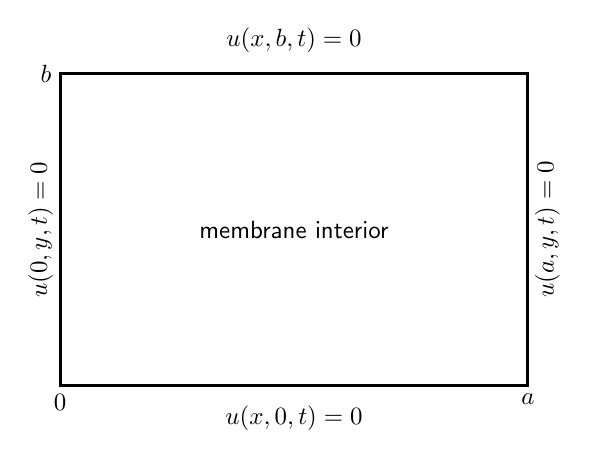
Figure 3. A rectangular membrane fixed on all four edges. The displacement vanishes on the entire boundary.

For a nontrivial separated mode,

X (0) = X (a) = 0.

(36)

The general x solution is

X = C cos(kxx ) + D sin(kxx ).

(37)

The condition X(0) = 0 gives C = 0.

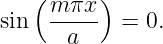
The condition X(a) = 0 requires

sin(kxa) = 0.

(38)

Thus

|------------------------------| k = m-π, m = 1,2,3,...| --x,m-----a----------------------

(39)

Similarly,

|----------------------------| | nπ | ky,n = ---, n = 1,2,3,...| --------b---------------------

(40)

Therefore the spatial mode is

|---------------(-----)----(-----)--| Φmn (x,y ) = sin m-πx- sin nπy- . | -------------------a----------b------

(41)

5 Why the mode indices begin at one

m = 0,

(42)

then the x sine factor vanishes everywhere.

n = 0,

(43)

then the y sine factor vanishes everywhere.

Thus zero indices do not produce nontrivial all-fixed rectangular membrane modes.

The lowest mode is

|------| |(1,1).| -------

(44)

6 Two-dimensional membrane spectrum

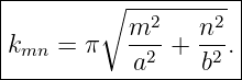
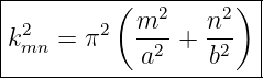
Since

k2mn = k2x,m + k2y,n,

(45)

|--------∘-----------| | m2 n2 | |kmn = π --2 + --2 . ------------a-----b---

(46)

Hence

|--------∘------------| | m2 n2 | ωmn = cπ -2-+ -2 ,| ------------a-----b----

(47)

and

|--------∘-----------| | c m2 n2 | |fmn = -- --2 + --2 . --------2---a-----b---

(48)

A single mode is therefore

|--------------------------------------------------| -umn-=--Φmn-(x,y)[Amn--cos(ωmnt)-+-Bmn-sin(ωmnt-)].|

(49)

7 Fundamental mode

For

(m, n) = (1,1),

(50)

( ) ( ) Φ11 = sin πx- sin πy- . a b

(51)

There are no interior nodal lines.

Only the four fixed edges are nodes.

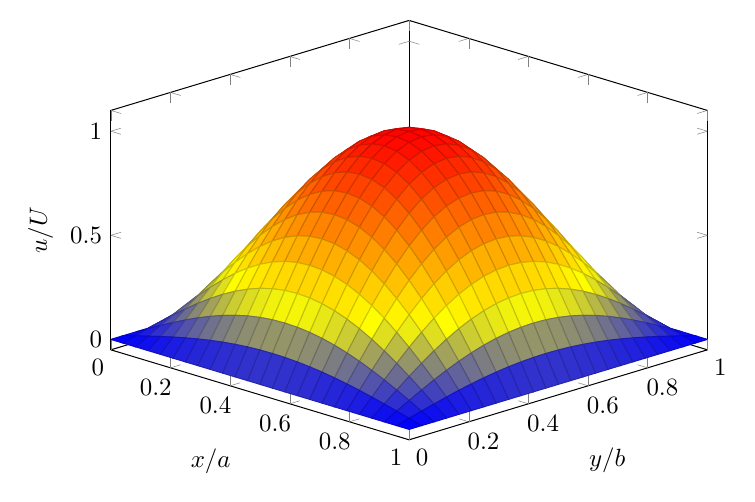
Figure 4. The (1,1) fundamental mode. The boundary is nodal and the membrane interior contains one antinodal region.

8 The (2,1) and (1,2) modes

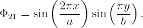
For the

(2,1)

(52)

mode,

( 2πx ) (πy ) Φ21 = sin ---- sin --- . a b

(53)

It has one interior vertical nodal line:

|------| x = a.| -----2--

(54)

For the

(1,2)

(55)

mode, the corresponding interior nodal line is

|------| | b-| y = 2.| --------

(56)

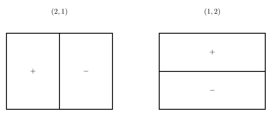
Figure 5. The (2,1) and (1,2) mode patterns. Increasing one index inserts nodal lines perpendicular to that coordinate direction.

9 General nodal-line positions

Vertical interior nodal lines satisfy

( ) sin mπx-- = 0. a

(57)

Thus

|--------------------------------| | ja- | |x = m , j = 1, 2,...,m − 1. | ---------------------------------

(58)

Horizontal interior nodal lines satisfy

|------------------------------| |y = ℓb, ℓ = 1,2,...,n − 1.| -----n--------------------------

(59)

A mode (m,n) therefore has:

m − 1 interior vertical nodal lines,
n − 1 interior horizontal nodal lines,
mn rectangular antinodal regions.

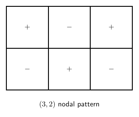
Figure 6. The (3,2) mode has two vertical interior nodal lines and one horizontal interior nodal line, producing six alternating antinodal regions.

10 Example 1: membrane wave speed

Take

2 𝒯 = 120 N ∕m, σ = 0.0300 kg∕m .

(60)

Then

c	=	(61)
	=	(62)
	≈ 63.25 m∕s.	(63)

11 Example 2: rectangular membrane fundamental

Let

a = 0.800 m, b = 0.600 m.

(64)

Using

c ≈ 63.25 m ∕s,

(65)

f₁₁	=	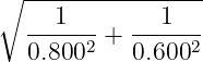(66)
	≈ 65.88 Hz.	(67)

12 Example 3: two higher modes

For

(2,1),

(68)

f₂₁	=	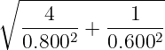(69)
	≈ 95.01 Hz.	(70)

For

(1,2),

(71)

f₁₂	=	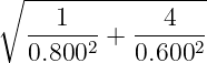(72)
	≈ 112.58 Hz.	(73)

Because

a ⁄= b,

(74)

the two frequencies differ.

13 Square membrane and degeneracy

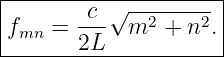
For a square,

a = b = L.

(75)

Then

|-------c-√----------| |fmn = --- m2 + n2.| -------2L-------------

(76)

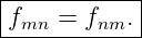
Interchanging the indices does not change the frequency:

|-----------| fmn-=--fnm.--

(77)

Thus for

m ⁄= n,

(78)

the distinct mode shapes

Φmn

(79)

and

Φnm

(80)

are degenerate.

Any linear combination of degenerate eigenfunctions is also an eigenfunction with the same eigenfrequency:

|----------------------| -Φ-=--C1Φmn--+-C2Φnm.--|

(81)

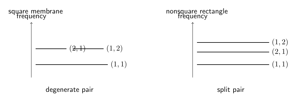
Figure 7. A square membrane has symmetry degeneracies because the frequency depends on m² + n². A nonsquare rectangle generally separates the (m,n) and (n,m) frequencies.

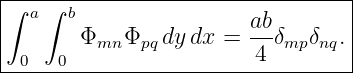
14 Orthogonality in each coordinate

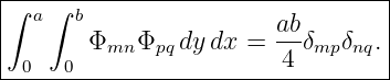
The sine functions satisfy

∫------------------------------------| | a ( m πx ) ( pπx ) a | | sin -a--- sin -a-- dx = 2-δmp.| --0-----------------------------------

(82)

Likewise,

∫------(-----)---(-----)------------| | b n-πy qπy- b- | | sin b sin b dy = 2δnq. | --0---------------------------------

(83)

Therefore

∫--a∫-b--------------------------| | Φmn Φpq dy dx = abδmpδnq.| --0--0------------------4---------

(84)

This two-dimensional orthogonality is what allows arbitrary initial shapes to be decomposed into independent membrane modes.

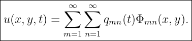
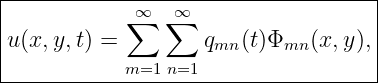
15 General modal expansion

The general ideal fixed-edge motion is

|-----------------------------------| | ∞∑ ∑∞ | u(x, y,t) = qmn (t)Φmn (x,y ). | | m=1 n=1 | -------------------------------------

(85)

Each modal coordinate obeys

|------------------| q¨mn-+--ω2mnqmn--=-0.-

(86)

Thus

|----------------------------------------| qmn (t) = Amn cos(ωmnt ) + Bmn sin (ωmnt).| ------------------------------------------

(87)

16 Initial displacement coefficients

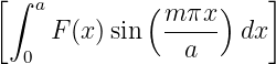
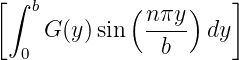
Let

u (x, y,0) = f(x,y).

(88)

Then

∑ f(x,y ) = A Φ (x, y). mn mn m,n

(89)

Project onto

Φpq

(90)

and use orthogonality:

|--------------------------------------------------| | 4 ∫ a ∫ b ( pπx ) (qπy ) | |Apq = --- f(x, y)sin ---- sin ---- dydx. | -------ab--0---0--------------a----------b----------

(91)

17 Initial velocity coefficients

Let

ut(x,y,0) = g(x, y).

(92)

Since

˙qmn(0) = ωmnBmn,

(93)

we obtain

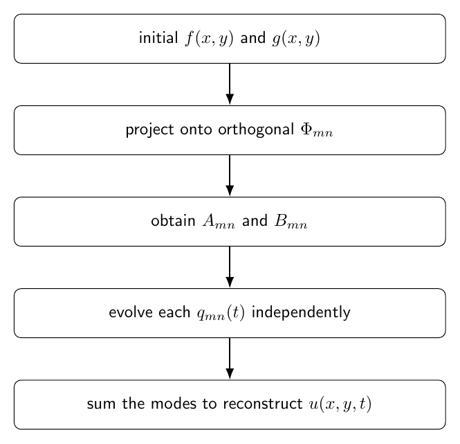
|------------------------------------------------------| | 4 ∫ a∫ b (p πx) ( qπy ) | |Bpq = ------ g(x,y) sin ---- sin ---- dy dx. | --------abωpq--0---0--------------a---------b----------|

(94)

Figure 8. Arbitrary initial displacement and velocity are projected onto the orthogonal membrane modes. Each resulting modal coordinate then evolves independently.

18 Example 4: initial shape equal to one mode

Let

(2 πx) ( 3πy) f(x, y) = U0sin ---- sin ---- , a b

(95)

with

g(x,y ) = 0.

(96)

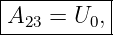
Orthogonality immediately gives

|----------| -A23-=-U0,-|

(97)

all other

Amn = 0,

(98)

and all

Bmn = 0.

(99)

Therefore

|--------------------------------| |u(x,y,t) = U0Φ23 (x,y)cos(ω23t).| ----------------------------------

(100)

A pure normal mode remains pure in the ideal linear system.

19 Separable initial shapes

f(x,y) = F (x)G (y),

(101)

then the coefficient factors:

A_mn	=	(102)
	×.	(103)

The two-dimensional Fourier coefficient becomes a product of two one-dimensional sine-series coefficients.

20 Normal modes as an eigenvalue problem

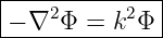
The spatial mode satisfies

|--------------| |− ∇2 Φ = k2Φ | ---------------

(104)

inside the rectangle, with

Φ = 0

(105)

on the boundary.

Thus

Φmn

(106)

are eigenfunctions and

|---------(----------)-| | 2 2 m2 n2 | |kmn = π --2 + -2- | -------------a----b----

(107)

are eigenvalues.

The membrane is therefore a continuous two-dimensional version of the normal-mode eigenvalue problem introduced in M06-05.

21 Modal energy

Each modal coordinate has the oscillator equation

q¨mn + ω2mnqmn = 0.

(108)

With a chosen mode normalization, its energy has the oscillator form

|------------------------------| | 1- eff [ 2 2 2 ] | Emn = 2M mn q˙mn + ω mnqmn .| --------------------------------

(109)

Orthogonality removes cross terms between distinct ideal normal modes.

22 Scaling with tension and surface density

Because

∘ --- c = 𝒯-, σ

(110)

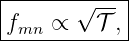
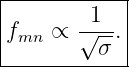
all modal frequencies satisfy

|-------√----| -fmn-∝----𝒯 ,|

(111)

and

|------------| |fmn ∝ √1-. | ----------σ--|

(112)

Thus multiplying tension by four doubles all modal frequencies.

Multiplying surface mass density by four halves all modal frequencies.

The ideal mode shapes remain unchanged because their geometry and boundary conditions have not changed.

23 Geometry and spectral splitting

Changing a or b affects the two spatial indices differently.

The term

m ∕a

(113)

depends on the horizontal dimension, while

n∕b

(114)

depends on the vertical dimension.

A square has extra symmetry and therefore systematic degeneracies.

Changing it into a rectangle generally splits those symmetry-related frequencies.

24 Limits of the ideal membrane model

The model assumes:

uniform isotropic tension,
uniform surface density,
negligible bending stiffness,
perfectly fixed edges,
small slopes and displacements,
linear response,
negligible damping.

Real membranes can have damping, nonuniform tension, material anisotropy, finite boundary compliance, and nonlinear large-amplitude behavior.

A circular drumhead also has different eigenfunctions.

Its radial equation produces Bessel functions rather than ordinary sines.

That is the subject of M06-18.

25 Common mistakes

Using string tension units N rather than membrane tension per unit length N∕m.
Using linear mass density instead of surface mass density.
Forgetting both spatial second derivatives in the membrane equation.
Treating one separated product as the most general motion.
Choosing positive separation constants that lead to exponentials instead of fixed-edge oscillatory eigenfunctions.
Allowing m = 0 or n = 0 for a membrane fixed on all four edges.
Writing k_mn = k_x + k_y rather than k_mn² = k_x² + k_y².
Forgetting the factor of π in the rectangular eigenvalues.
Miscounting interior nodal lines.
Assuming (m,n) and (n,m) are degenerate for every rectangle.
Forgetting that any linear combination of degenerate eigenfunctions stays in the same eigenspace.
Forgetting the normalization factor 4∕(ab) in the modal coefficients.
Treating arbitrary initial displacement as one mode.
Assuming changing tension changes the ideal spatial mode shapes.
Using rectangular sine modes for a circular membrane.

26 Practice exercises

Derive the membrane wave equation from a small rectangular element.
Verify dimensionally that 𝒯 ∕σ has units of speed squared.
Substitute u = XY Q into the membrane PDE and obtain the separated equations.
Derive k_x,m = mπ∕a from fixed-edge conditions.
Derive k_y,n = nπ∕b.
Derive the complete frequency formula f_mn.
Locate the nodal lines of a (4, 3) mode.
Reproduce Examples 1 through 3 numerically.
Show that (2, 1) and (1, 2) are degenerate on a square membrane.
Construct two different linear combinations of those degenerate square-membrane modes.
Prove the two-dimensional orthogonality relation.
Derive the initial-displacement coefficient formula.
Derive the initial-velocity coefficient formula.
Show how the coefficient factors when f(x,y) = F(x)G(y).
Explain why increasing tension changes frequencies but not ideal mode shapes.

27 Summary

The ideal uniform membrane obeys

|---------------------| σu = 𝒯 (u + u ), | ---tt-------xx----yy----

(115)

with

|----∘-----| | 𝒯 | |c = --.| --------σ--

(116)

For a fixed rectangular membrane,

|---------------(-----)----(-----)--| Φmn (x,y ) = sin m-πx- sin nπy- , | -------------------a----------b------

(117)

and

|--------∘-----------| | c m2 n2 | |fmn = -- --2 + --2 . --------2---a-----b---

(118)

The modes obey

|--------------------------------| ∫ a∫ b ab | | Φmn Φpq dy dx = --δmpδnq.| --0--0------------------4---------

(119)

General motion is

|-----------∞∑--∑∞-------------------| u(x, y,t) = q (t)Φ (x,y ), | | mn mn | -----------m=1-n=1-------------------

(120)

with

|-------2----------| q¨mn-+--ωmnqmn--=-0.-

(121)

Separation of variables therefore converts one two-dimensional field equation into a discrete family of independent harmonic oscillators.

References

[1] PhysicsLibrary, M06-16, Wave Equations in Two and Three Dimensions and Spherical Waves.

[2] PhysicsLibrary, M06-08, Continuous Strings, Standing Waves, and Normal Modes.

[3] PhysicsLibrary, M06-05, Small Oscillations and the Normal-Mode Eigenvalue Problem.

[4] A. P. French, Vibrations and Waves, W. W. Norton, 1971.

[5] G. B. Arfken, H. J. Weber, and F. E. Harris, Mathematical Methods for Physicists, 7th ed., Academic Press, 2013.

"Separation of Variables, Membranes, and Two-Dimensional Normal Modes" is owned by bloftin.
(view preamble)

Separation of Variables, Membranes, and Two-Dimensional Normal Modes