Small Oscillations and the Normal-Mode Eigenvalue Problem
Many mechanical systems are nonlinear when written exactly.
Near a stable equilibrium, however, their motion often simplifies dramatically.
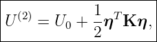
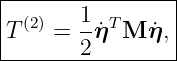
To second order in small displacements, a broad class of conservative systems takes the
form
Here
- η is the displacement from equilibrium in generalized coordinates,
- M is the mass matrix evaluated at equilibrium,
- K is the stiffness matrix, equal to the Hessian of the potential at equilibrium.
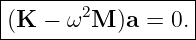
The associated normal modes satisfy
This is the generalized normal-mode eigenvalue problem.
Its eigenvalues
determine the small-oscillation frequencies, while its eigenvectors determine the collective mode
shapes.
M06-04 introduced this structure using coupled springs.
The present article derives it from the local mechanics of a general conservative system and
develops the mathematical properties that make modal analysis work.
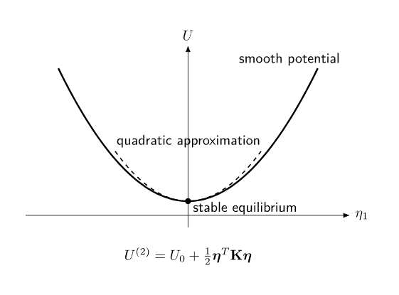
Figure 1. Near a stable equilibrium, a smooth potential surface is approximated by a quadratic
form. Its local curvature determines the stiffness matrix and therefore the small-oscillation
frequencies.
1 Equilibrium and displacement coordinates
Let the system have generalized coordinates
Suppose
is an equilibrium configuration.
Define the small displacement vector
At equilibrium,
for every independent coordinate.
This removes the linear term from the local expansion of the potential energy.
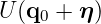
2 Quadratic expansion of the potential
Expand
in a Taylor series:
| U | = U0 + ∑
i 0ηi 0ηi | (9)
|
| +  ∑
i,j ∑
i,j 0ηiηj + 0ηiηj +  . . | (10) |
The first derivatives vanish at equilibrium.
Therefore, to quadratic order,
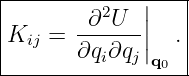
where
The matrix
is the Hessian of the potential at equilibrium.
For a smooth potential,
3 Stable equilibrium and the stiffness matrix
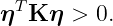
For a strict stable equilibrium, the quadratic change in potential must be positive for every
nonzero sufficiently small displacement:
Thus, in the nondegenerate stable case,
If
is only positive semidefinite, zero-curvature directions can occur.
These directions lead to zero modes.
If the quadratic form has a negative direction, the equilibrium is linearly unstable.
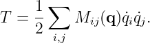
4 Quadratic kinetic energy
For a broad class of mechanical systems,
Near equilibrium,
The velocities are already first order in the small motion.
Therefore replacing
by its equilibrium value introduces only higher-order corrections.
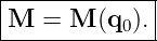
To quadratic order,
where
For independent physical degrees of freedom,
and normally
5 Why coordinate-dependent inertia can be frozen at equilibrium
Suppose
The correction
is first order in
But
contains one factor of displacement and two factors of velocity.
It is third order in the small-motion bookkeeping.
Therefore it is omitted in the quadratic small-oscillation theory.
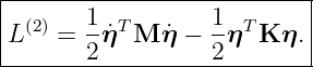
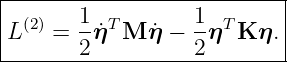
6 Quadratic Lagrangian
Ignoring the irrelevant constant
the quadratic Lagrangian is
The Euler-Lagrange equations give
This is the universal linear system for conservative small oscillations.
7 Normal-mode ansatz
Seek a collective motion
Then
Substitution yields
For a nonzero mode vector,
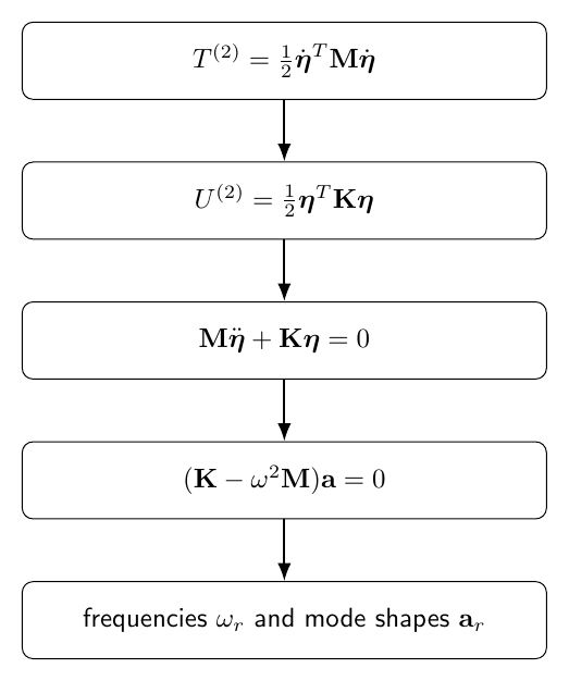
Figure 2. The quadratic kinetic and potential energies define M and K. The small-oscillation
equations then reduce to a generalized eigenvalue problem whose eigenvalues are ω2 and whose
eigenvectors are mode shapes.
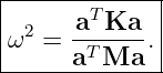
8 Why the eigenvalues are frequencies squared
The generalized eigenvalue equation is
Comparison with the mode equation identifies
Thus a positive eigenvalue gives an oscillatory angular frequency
A zero eigenvalue gives a zero mode.
A negative eigenvalue corresponds to an imaginary
and therefore exponential behavior rather than stable oscillation.
9 Rayleigh quotient
Multiply
on the left by
Then
Therefore any exact mode satisfies
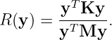
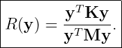
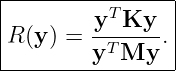
This ratio motivates the Rayleigh quotient
The normal modes are stationary directions of this quotient.
For a positive-definite conservative system, the lowest mode minimizes the Rayleigh
quotient.
10 Reality and positivity of stable frequencies
If
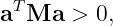
is positive definite and
is positive definite, then for every nonzero
and
Hence
The mass-weighting transformation below also shows that the eigenvalues are real.
11 Mass-weighted coordinates
Because
is positive definite, it has a positive square root
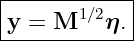
Define
Then
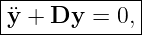
The equation of motion becomes
where
Since
and
are symmetric,
Thus the generalized eigenvalue problem becomes an ordinary symmetric eigenvalue
problem.
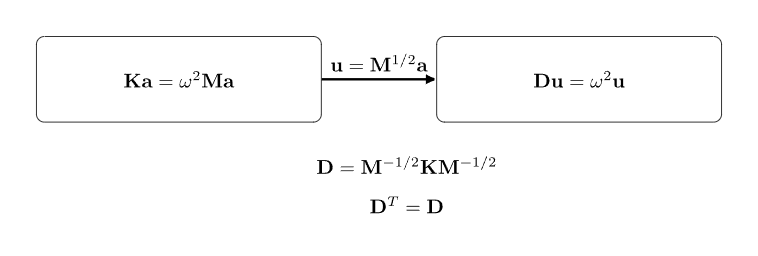
Figure 3. Mass weighting converts the generalized problem Ka = ω2Ma into an ordinary
symmetric eigenvalue problem for D = M−1∕2KM−1∕2.
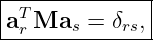
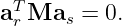
12 Orthogonality of distinct modes
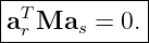
Let
and
satisfy
and
Multiply the first equation by
and the second by
Using symmetry,
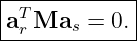
Therefore
For distinct eigenfrequencies,
Distinct modes are orthogonal in the mass inner product.
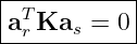
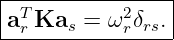
13 Stiffness orthogonality
For distinct mass-orthogonal modes,
Therefore
when
and the frequencies are distinct.
Thus normal modes diagonalize both quadratic forms.
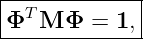
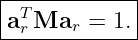
14 Mass normalization
The scale of an eigenvector is arbitrary.
A particularly useful convention is
Then
and
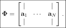
15 Modal matrix and simultaneous diagonalization
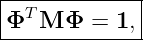
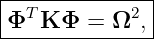
Collect the mass-normalized mode vectors into
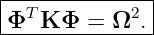
Then
and
where
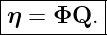
Set
Then
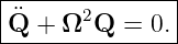
The coupled small-oscillation system becomes a collection of independent harmonic
oscillators.
16 Quadratic energy in normal coordinates
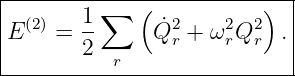
The quadratic energy is
Use
For mass-normalized modes,
Each normal coordinate carries the energy of an independent SHO.
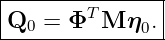
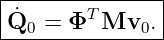
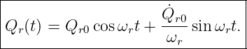
17 Projecting arbitrary initial conditions
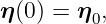
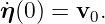
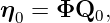
Suppose
and
Since
multiply by
Using mass normalization,
Similarly,
For every positive-frequency mode,
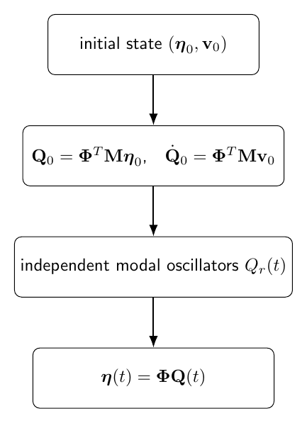
Figure 8. Initial displacement and velocity are projected onto the mass-normalized mode basis.
Each modal initial state then evolves independently as a one-dimensional harmonic oscillator.
18 Degenerate normal frequencies
Two or more linearly independent modes can share the same frequency.
This is a degeneracy.
If
the earlier orthogonality proof does not force
However, within the degenerate eigenspace, one can choose a mass-orthonormal basis.
Thus degeneracy means the mode basis is not unique.
Any suitable linear combination within the degenerate eigenspace is also a mode with the same
frequency.
19 Zero modes
If
then
The potential has no quadratic restoring curvature in that direction.
The modal equation becomes
Therefore
A zero mode is not an oscillator.
It represents a neutral direction, often associated with a continuous symmetry.
20 Unstable modes
Suppose an eigenvalue is negative:
Then the modal equation is
Its solution is
The growing exponential signals linear instability.
Thus the spectrum of the quadratic problem classifies local behavior:
- ω2 > 0: stable oscillatory mode,
- ω2 = 0: neutral zero mode,
- ω2 < 0: unstable mode.
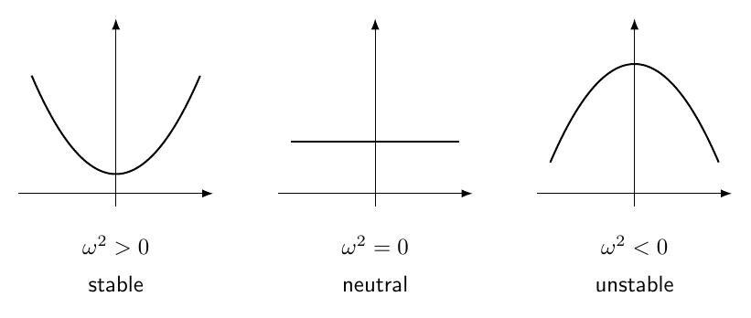
Figure 7. The sign of the generalized eigenvalue classifies the local motion: positive eigenvalues
give oscillations, zero eigenvalues give neutral directions, and negative eigenvalues give
exponentially growing and decaying solutions.
21 Example 1: equal-mass double pendulum
Consider a planar double pendulum with:
- two equal point masses m,
- two massless rods of equal length ℓ,
- small angular displacements 𝜃1 and 𝜃2 from the downward vertical.
The exact kinetic energy is
| T | =  mℓ2 mℓ2 2𝜃12 + 𝜃
22 2𝜃12 + 𝜃
22 | (100)
|
| + 2𝜃1𝜃2 cos(𝜃1 − 𝜃2)![]](https://images.physicslibrary.org/cache/objects/1496/make4ht/SmallOscillationsAndTheNormalModeEigenvalueProblem103x.png) . . | (101) |
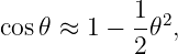
For small oscillations,
Thus
The gravitational potential is
Using
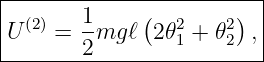
the quadratic part is
apart from an additive constant.
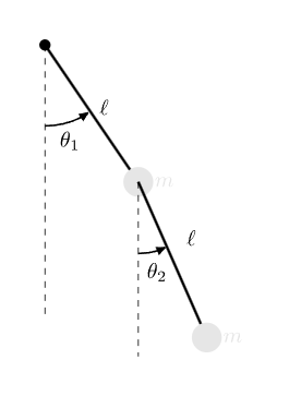
Figure 4. Small angles 𝜃1 and 𝜃2 describe the double pendulum near its downward equilibrium.
The kinetic energy couples the angular velocities even though the quadratic gravitational stiffness
matrix is diagonal in these coordinates.
22 Double-pendulum mass and stiffness matrices
Define
Then
and
This example is important because
is not diagonal.
Coupling can arise through kinetic energy as well as potential energy.
23 Double-pendulum eigenvalue equation
The mode condition is
Define the dimensionless quantity
Then
Thus
Therefore
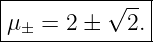
The roots are
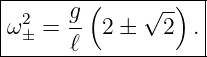
Hence
24 Double-pendulum mode shapes
For the lower frequency,
The eigenvector equation gives
The two angles have the same sign.
For the higher frequency,
and
The two angles have opposite signs.
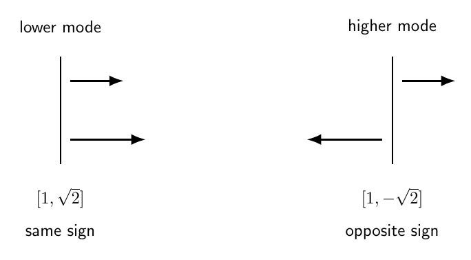
Figure 5. The equal-mass double pendulum has a lower-frequency same-sign angular mode and a
higher-frequency opposite-sign mode. The relative amplitude magnitude is  in these angular
coordinates.
in these angular
coordinates.
25 Example 2: numerical double-pendulum frequencies
Let
Then
| ω− | = 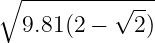 | (123)
|
| ≈ 2.40 rad∕s, | (124) |
and
| ω+ | = 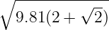 | (125)
|
| ≈ 5.79 rad∕s. | (126) |
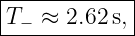
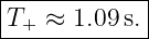
The corresponding periods are approximately
and
26 Example 3: Rayleigh estimate of the lowest double-pendulum frequency
Choose the simple trial direction
The Rayleigh quotient is
For the double pendulum,
while
Therefore
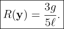
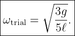
The trial estimate is
The exact lowest squared frequency is
The trial value is
which is already close.
This illustrates why the Rayleigh quotient is useful for estimating low modes of systems whose
exact eigenproblem is difficult.
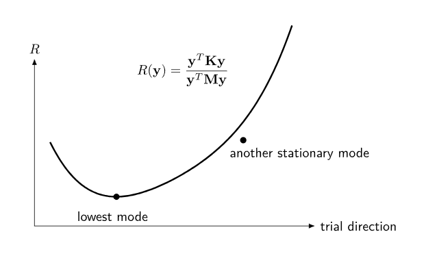
Figure 6. The Rayleigh quotient assigns an effective squared frequency to any trial direction. Its
stationary directions are the normal modes, and its minimum gives the lowest mode for a
positive-definite conservative system.
27 Coordinate changes and physical invariance
Let
for an invertible constant matrix
Then
and
transform by congruence:
and
The component form changes, but the physical Normal frequencies do not.
Thus normal frequencies are properties of the local mechanical system, not artifacts of a particular
generalized-coordinate basis.
28 Degeneracy and symmetry
Degenerate frequencies frequently reflect symmetry.
For example, an isotropic two-dimensional oscillator has equal stiffness in two independent
directions.
Its two mode frequencies are equal.
Within that two-dimensional eigenspace, many different orthogonal pairs can be chosen as mode
shapes.
Symmetry therefore often explains both degeneracy and freedom in the choice of mode
basis.
29 Beyond the quadratic approximation
The small-oscillation theory neglects cubic and higher terms such as
At larger amplitude these terms can produce:
- amplitude-dependent frequencies,
- coupling between normal modes,
- internal Resonances,
- nonlinear energy transfer,
- chaotic behavior in sufficiently nonlinear systems.
Normal modes are exact for the quadratic linearized system and approximate for the original
nonlinear system near equilibrium.
30 Why the theory is so general
The same generalized eigenvalue structure appears in:
- molecular vibrations,
- structural vibration analysis,
- lattice dynamics,
- acoustic cavities,
- elastic bodies,
- finite-element models,
- electrical small-signal systems,
- wave equations after spatial discretization.
The normal-mode eigenproblem is therefore one of the central mathematical structures linking
classical mechanics to much broader physics.
31 Common mistakes
- Expanding about a configuration that is not an equilibrium.
- Keeping the linear term in the potential even though the expansion point is an
equilibrium.
- Treating the mass matrix as automatically diagonal in generalized coordinates.
- Forgetting that coordinate dependence of M contributes only beyond quadratic order
in the standard small-oscillation expansion.
- Solving det K = 0 instead of det(K − ω2M) = 0.
- Interpreting the generalized eigenvalue itself as ω rather than ω2.
- Using ordinary Euclidean orthogonality when the mass matrix is not proportional to
the identity.
- Forgetting that eigenvectors have arbitrary overall scale.
- Forgetting to mass normalize before using Q = ΦT Mη.
- Applying the positive-frequency SHO formula to a zero mode.
- Calling a negative eigenvalue an oscillation frequency instead of recognizing an
instability.
- Assuming degenerate mode vectors are unique.
- Confusing a diagonal stiffness matrix with a fully decoupled problem when the mass
matrix is not diagonal.
- Assuming normal modes exchange energy in the exact conservative quadratic theory.
- Extending the quadratic approximation to amplitudes where higher-order terms are
no longer negligible.
32 Practice exercises
- Starting from a Taylor expansion of U, derive the quadratic stiffness matrix.
- Explain why the first derivatives of the potential vanish at equilibrium.
- Show why coordinate dependence of the mass matrix can be neglected to quadratic
order.
- Derive the small-oscillation equations from the quadratic Lagrangian.
- Derive the generalized normal-mode eigenvalue problem.
- Prove mass orthogonality of distinct modes.
- Show that distinct modes are also stiffness orthogonal.
- Derive the mass-weighted symmetric matrix D.
- Derive the modal projection formulas for initial displacement and velocity.
- Derive the modal energy as a sum of independent oscillator energies.
- Explain the difference among positive, zero, and negative eigenvalues.
- Derive the double-pendulum mass and stiffness matrices.
- Solve the double-pendulum characteristic equation and mode shapes.
- Reproduce the numerical double-pendulum frequencies for ℓ = 1 m.
- Use the Rayleigh quotient with a trial vector of your choice and compare the estimate
with an exact normal frequency.
33 Summary
Near a stable equilibrium, a conservative mechanical system has the quadratic Lagrangian
The equations of motion are
Normal modes satisfy
Distinct modes obey
With mass-normalized modes,
and
The Rayleigh quotient is
Positive eigenvalues give stable oscillations, zero eigenvalues give neutral modes, and negative
eigenvalues indicate linear instability.
The next step is to apply this finite-dimensional mode theory to extended discrete systems, where
a chain of oscillators develops a dispersion relation and begins to behave like a wave-bearing
medium.
References
References
[1] PhysicsLibrary, M06-04, Coupled Oscillators and Normal Modes.
[2] PhysicsLibrary, M06-03, Driven Harmonic Motion and Resonance.
[3] PhysicsLibrary, M06-01, Simple Harmonic Motion.
[4] A. P. French, Vibrations and Waves, W. W. Norton, 1971.
[5] J. R. Taylor, Classical Mechanics, University Science Books, 2005.
[6] H. Goldstein, C. Poole, and J. Safko, Classical Mechanics, 3rd ed., Addison-Wesley,
2002.



























































![|--------------------------------|
| (2) 1 2[ 2 2] |
|T = -m ℓ 2˙𝜃1 + 2 ˙𝜃1 ˙𝜃2 + 𝜃˙2 .
--------2------------------------](https://images.physicslibrary.org/cache/objects/1496/make4ht/SmallOscillationsAndTheNormalModeEigenvalueProblem105x.png)

![[ ]
𝜃1
𝜃 = 𝜃 .
2](https://images.physicslibrary.org/cache/objects/1496/make4ht/SmallOscillationsAndTheNormalModeEigenvalueProblem109x.png)
![|------------------|
| [ ] |
|M = m ℓ2 2 1 ,|
------------1--1---](https://images.physicslibrary.org/cache/objects/1496/make4ht/SmallOscillationsAndTheNormalModeEigenvalueProblem110x.png)
![|------------------|
| [2 0] |
|K = mg ℓ . |
------------0--1---](https://images.physicslibrary.org/cache/objects/1496/make4ht/SmallOscillationsAndTheNormalModeEigenvalueProblem111x.png)



![[[ ] [ ]]
det 2 0 − μ 2 1 = 0.
0 1 1 1](https://images.physicslibrary.org/cache/objects/1496/make4ht/SmallOscillationsAndTheNormalModeEigenvalueProblem115x.png)



![|-----[---]--|
| √1-- |
|a− ∝ 2 .|
--------------](https://images.physicslibrary.org/cache/objects/1496/make4ht/SmallOscillationsAndTheNormalModeEigenvalueProblem121x.png)

![|-----[-----]--|
| 1 |
|a+ ∝ − √2- .|
----------------](https://images.physicslibrary.org/cache/objects/1496/make4ht/SmallOscillationsAndTheNormalModeEigenvalueProblem123x.png)

![[1]
y = .
1](https://images.physicslibrary.org/cache/objects/1496/make4ht/SmallOscillationsAndTheNormalModeEigenvalueProblem130x.png)