ED02: Vectors, Fields, and Coordinate Geometry
Electrodynamics is written in the language of vector fields. Before deriving Coulomb’s law, Gauss’s
Law, the Biot-Savart law, or Maxwell’s equations in detail, we need a precise geometric language
for direction, magnitude, components, position, and spatial variation.
The central lesson of this article is that a vector is not the same thing as its list of components.
The vector is the geometric object. Components are the numbers used to describe that object
relative to a chosen basis.
That distinction becomes especially important in cylindrical and spherical coordinates, where the
basis directions themselves change from point to point.
This article therefore develops the coordinate geometry that later electrodynamics will repeatedly
use:
- vectors and scalars,
- basis vectors and components,
- dot and cross products,
- position and displacement vectors,
- scalar and vector fields,
- orthogonal curvilinear coordinates,
- scale factors,
- Cartesian, cylindrical, and spherical bases,
- and differential line, area, and volume elements.
Gradient, divergence, and curl are intentionally deferred to ED03. Here the emphasis is the
geometry from which those operators will later be derived.
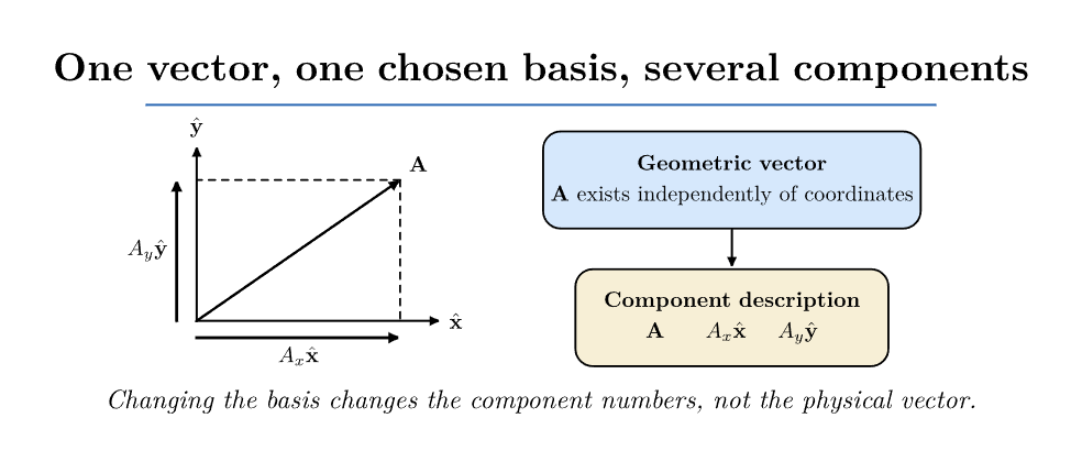
Figure 1. A geometric vector is independent of the coordinate description used to represent it.
Once a basis is chosen, the vector can be decomposed into components along the basis directions.
1 Scalars and vectors
A scalar is a quantity specified by a magnitude, possibly with units, but without an intrinsic
spatial direction.
Examples include
A vector has both magnitude and direction.
Examples include
A geometric vector can be represented by a directed line segment. If A is a vector, its magnitude is
written
The zero vector has zero magnitude:
Unlike an ordinary number, a vector cannot in general be characterized by magnitude
alone.
2 Vectors versus components
Choose an orthonormal Cartesian basis
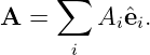
Any vector A can be written
The numbers
are the components of A in that basis.
If we rotate the coordinate axes, the vector itself does not change, but the components generally
do.
This is a fundamental distinction:
The same physical Electric Field can therefore have different component triples in different
coordinate systems while representing the same field at the same physical point.
Magnitude from components
Because the Cartesian basis is orthonormal,
with analogous relations for the other basis vectors.
Therefore
so
3 Vector addition and scalar multiplication
If
and
then
For scalar c,
Vector addition is geometric. Components make the calculation convenient, but the parallelogram
or head-to-tail rule gives the underlying geometric meaning.
4 The dot product
For vectors A and B separated by angle 𝜃,
The dot product produces a scalar.
In an orthonormal Cartesian basis,
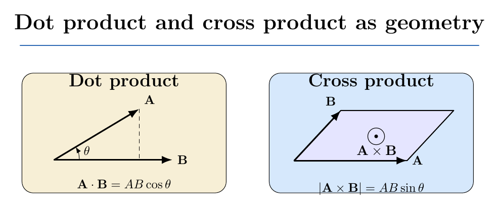
Figure 2. The dot product measures parallel alignment through a projection, while the cross
product measures oriented perpendicular content through the area of the parallelogram spanned
by the two vectors.
Projection
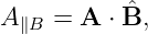
The scalar component of A along B is
where
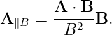
The corresponding vector projection is
Equivalently,
This same projection idea will later appear in electric flux, magnetic flux, work, boundary
conditions, polarization, and wave decomposition.
Orthogonality
If two nonzero vectors are perpendicular,
then
Thus the dot product is an algebraic test for orthogonality.
5 The cross product
The cross product is defined geometrically by
with direction perpendicular to the plane containing A and B according to the right-hand
rule.
Thus
where n is the oriented unit Normal.
The order matters:
For a right-handed Cartesian basis,
| x ×y | = z, | (27)
|
| y ×z | = x, | (28)
|
| z ×x | = y. | (29) |
Reversing any pair changes the sign.
Cartesian component form
Expanding bilinearly gives
| A × B = | (AyBz − AzBy)x | (30)
|
| + (AzBx − AxBz)y | (31)
|
| + (AxBy − AyBx)z. | (32) |
This expression should not obscure the geometric meaning: the cross product represents oriented
area and a normal direction.
6 Triple products
The scalar triple product is
Its magnitude equals the volume of the parallelepiped generated by the three vectors.
Cyclic permutations leave it unchanged:
Interchanging two vectors reverses the sign.
The Vector Triple Product satisfies
Equation (35) is often remembered as the BAC-CAB identity, but it is safer to recognize its
structural form: the result lies in the plane spanned by B and C.
7 Position and displacement vectors
Choose an origin O.
The position vector of point P is
In Cartesian coordinates,
If a second point has position r′, the displacement from the source point r′ to the field point r
is
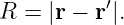
Its magnitude is
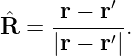
The corresponding unit vector is
This source-to-field-point geometry will appear constantly in Coulomb, Biot-Savart,
Green-function, multipole, and radiation integrals.
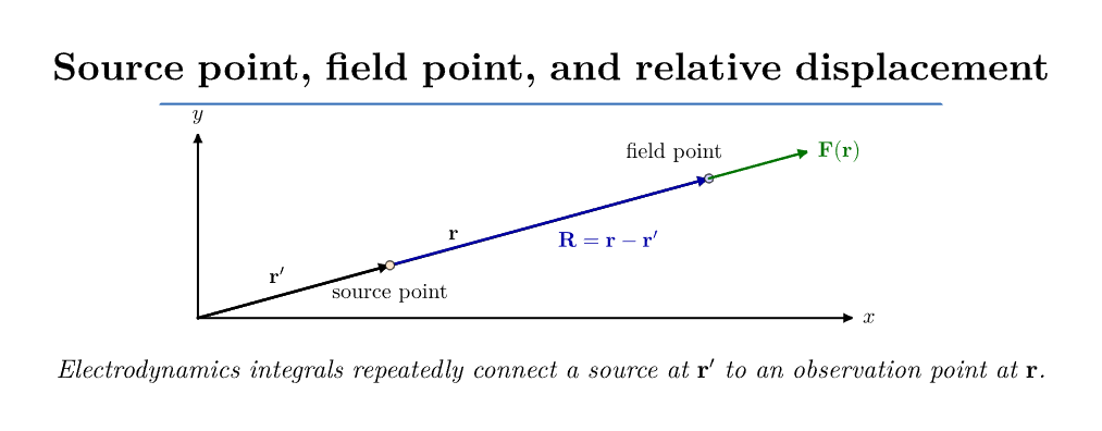
Figure 3. Position and displacement geometry. Electrodynamics repeatedly distinguishes the
source point r′ from the field point r. The relative vector R = r − r′ points from source to
observation point.
8 A vector field is not one vector
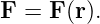
A vector field assigns a vector to each point in space:
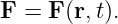
If time dependence is included,
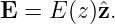
For example,
means that every spatial point has its own electric-field vector.
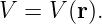
A scalar field instead assigns one scalar value to each point:
Electric potential is a scalar field; electric field is a vector field.
This difference becomes important in EDL03. A potential map consists of measured scalar values
V (x,y) on a grid. From spatial variation of that scalar field we will later infer a vector field
E.
9 Coordinate systems as geometric maps
A coordinate system assigns numbers to spatial points.
In Cartesian coordinates,
labels a point.
In cylindrical coordinates,
labels the same physical space.
In spherical coordinates,
provides another labeling.
The coordinate system is not the physical space itself. It is a description adapted to geometry and
symmetry.
This is why coordinate choice matters in electrodynamics. A spherical charge distribution is
usually easiest in spherical coordinates, a long straight wire in cylindrical coordinates, and a
rectangular electrode arrangement in Cartesian coordinates.
10 General orthogonal curvilinear coordinates
Let three coordinates be
The position vector is a function
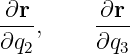
Hold q2 and q3 fixed while varying q1. This traces a coordinate curve.
The tangent to that curve is
Similarly,
point along the other coordinate curves.
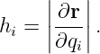
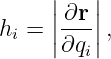
Define the scale factors
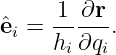
Then the corresponding unit vectors are
For an orthogonal coordinate system,
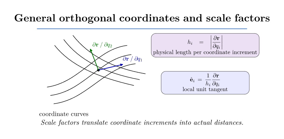
Figure 4. General orthogonal coordinates. Varying one coordinate while holding the others fixed
traces a coordinate curve. The derivative of the position vector along that curve gives a tangent
direction and its magnitude defines the scale factor hi.
11 Deriving the differential line element
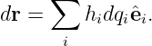
Differentiate Equation (49):
Using Equations (52) and (53),
For orthogonal coordinates,
The scale factors therefore convert coordinate increments into physical lengths.
This interpretation is crucial. A change dϕ is an angle, not a physical distance. The corresponding
physical arc length depends on where the point is located.
12 Differential area elements
Consider a small surface on which q1 is constant.
The two tangent edge vectors are
and
Their cross product gives the oriented area element:
For a right-handed orthogonal basis,
Cyclically,
| da2 | = h3h1 dq3dq1 e2, | (62)
|
| da3 | = h1h2 dq1dq2 e3. | (63) |
These formulas will later become the geometric foundation of electric and magnetic flux
integrals.
13 Differential volume element
The small coordinate cell has edge lengths
Therefore its differential volume is
This is the origin of factors such as
in cylindrical volume elements and
in spherical volume elements. They are geometric scale factors, not arbitrary memorized
corrections.
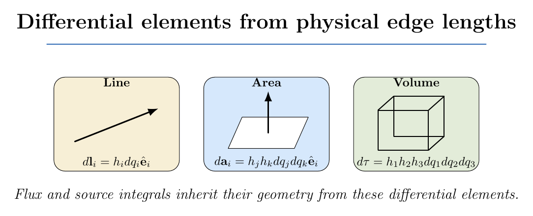
Figure 5. Differential line, area, and volume elements are built from the physical edge lengths of
an infinitesimal coordinate cell. The scale factors encode how coordinate increments become
actual distances.
14 Cartesian coordinates derived from the general construction
The Cartesian position vector is
Therefore
and
Hence
Thus
and
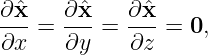
The Cartesian basis vectors are spatially constant:
with analogous results for y and z.
This simplicity is special. It does not hold for cylindrical or spherical unit vectors.
15 Cylindrical coordinates
Use cylindrical coordinates
where s is distance from the z axis, ϕ is azimuthal angle, and z is the usual Cartesian
height.
The coordinate transformation is
| x | = s cos ϕ, | (77)
|
| y | = s sin ϕ, | (78)
|
| z | = z. | (79) |
Therefore
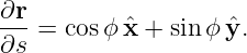
Differentiate with respect to s:
Its magnitude is unity, so
and
Differentiate Equation (80) with respect to ϕ:
Its magnitude is
Therefore
Finally,
so
Thus the cylindrical scale factors are
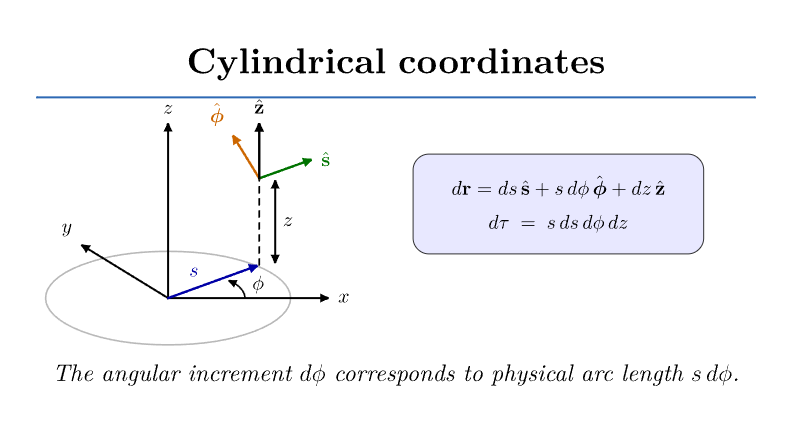
Figure 6. Cylindrical coordinates. The radial direction s and azimuthal direction ϕ rotate with
position. An angular increment dϕ corresponds to physical arc length sdϕ.
Cylindrical line element
Substituting Equation (89) into Equation (56),
The scalar distance element is
Cylindrical area elements
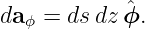
For a surface of constant s,
For a surface of constant ϕ,
For a surface of constant z,
Cylindrical volume element
Using Equation (65),
The factor s appears because an angular step dϕ spans a longer physical distance at larger
radius.
16 The cylindrical basis changes with position
Differentiate Equation (83) with respect to ϕ:
Similarly,
Therefore a vector field can vary even when its cylindrical components appear numerically
constant.
For example,
has constant radial component F0, but the direction of the vector changes around the
axis.
This basis variation is one of the main reasons divergence and curl formulas contain
geometry-dependent terms in curvilinear coordinates.
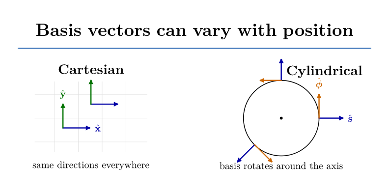
Figure 7. Basis-vector variation. Cartesian basis vectors keep the same direction everywhere,
while cylindrical and spherical basis vectors rotate as the observation point moves. Curvilinear
components cannot be differentiated as though the basis were constant.
17 Spherical coordinates
Use spherical coordinates
with r radial distance, 𝜃 polar angle measured from +z, and ϕ azimuthal angle about the z
axis.
The coordinate transformation is
| x | = r sin 𝜃 cos ϕ, | (100)
|
| y | = r sin 𝜃 sin ϕ, | (101)
|
| z | = r cos 𝜃. | (102) |
Hence
| r = | r sin 𝜃 cos ϕx + r sin 𝜃 sin ϕy | (103)
|
| + r cos 𝜃 z. | (104) |
Differentiate with respect to r:
 = | sin 𝜃 cos ϕx + sin 𝜃 sin ϕy | (105)
|
| + cos 𝜃 z. | (106) |
Its magnitude is unity, so
and
| r = | sin 𝜃 cos ϕx + sin 𝜃 sin ϕy | (108)
|
| + cos 𝜃 z. | (109) |
Differentiate Equation (104) with respect to 𝜃:
 = | r cos 𝜃 cos ϕx + r cos 𝜃 sin ϕy | (110)
|
| − r sin 𝜃 z. | (111) |
Its magnitude is r, so
and
| 𝜃 = | cos 𝜃 cos ϕx + cos 𝜃 sin ϕy | (113)
|
| − sin 𝜃 z. | (114) |
Finally,
 = | − r sin 𝜃 sin ϕx | (115)
|
| + r sin 𝜃 cos ϕy. | (116) |
Its magnitude is
Therefore
The spherical scale factors are therefore
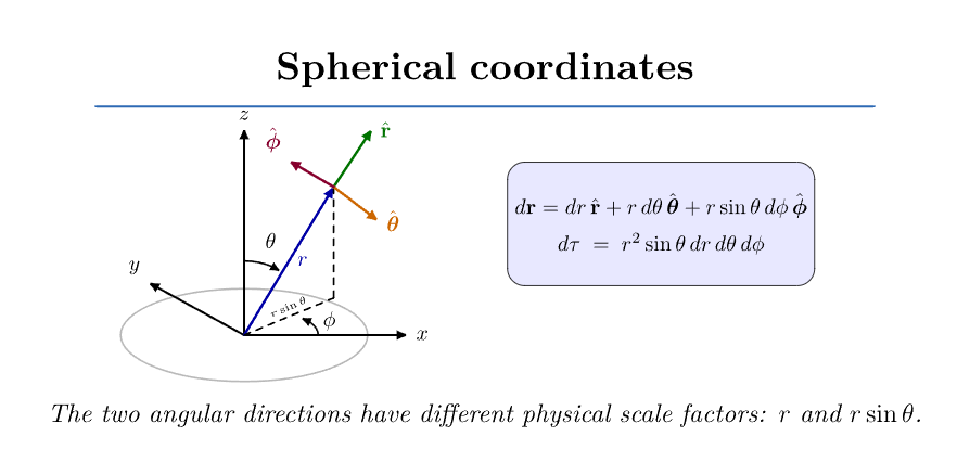
Figure 8. Spherical coordinates. At fixed radius, changing 𝜃 moves along a meridian with physical
length rd𝜃, while changing ϕ moves along a latitude circle with physical length r sin𝜃dϕ.
Spherical line element
Using Equation (119),
Thus
Spherical area elements
At constant r,
At constant 𝜃,
At constant ϕ,
Spherical volume element
The differential volume is
The factor r2 sin 𝜃 follows directly from the three physical edge lengths
18 Coordinate singularities are descriptive, not necessarily physical
Cylindrical coordinates become singular on the axis
because the azimuthal angle ϕ becomes undefined there.
Spherical coordinates become singular at
and along the polar axis where
A coordinate singularity does not automatically indicate a physical singularity.
For example, a perfectly finite uniform electric field can be expressed in spherical components that
have awkward angular behavior near the poles. The underlying physical field may remain smooth
even when the coordinate description becomes degenerate.
This distinction will become important when interpreting field singularities near point charges
versus harmless singularities introduced by coordinate choice.
19 Electrodynamics examples of symmetry-adapted coordinates
Coordinate systems are most powerful when they match the symmetry of the source.
Point charge
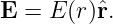
A point charge at the origin produces an electric field whose direction is radial:
Spherical coordinates expose this symmetry immediately.
Infinite line charge
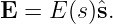
For an ideal line charge along the z axis,
Cylindrical coordinates make the radial dependence explicit.
Long straight current
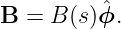
For an ideal current along the z axis, the magnetic field circles the wire:
Again, cylindrical coordinates align with the field geometry.
Parallel plates
Between large ideal parallel plates with negligible edge effects,
Cartesian coordinates are natural.
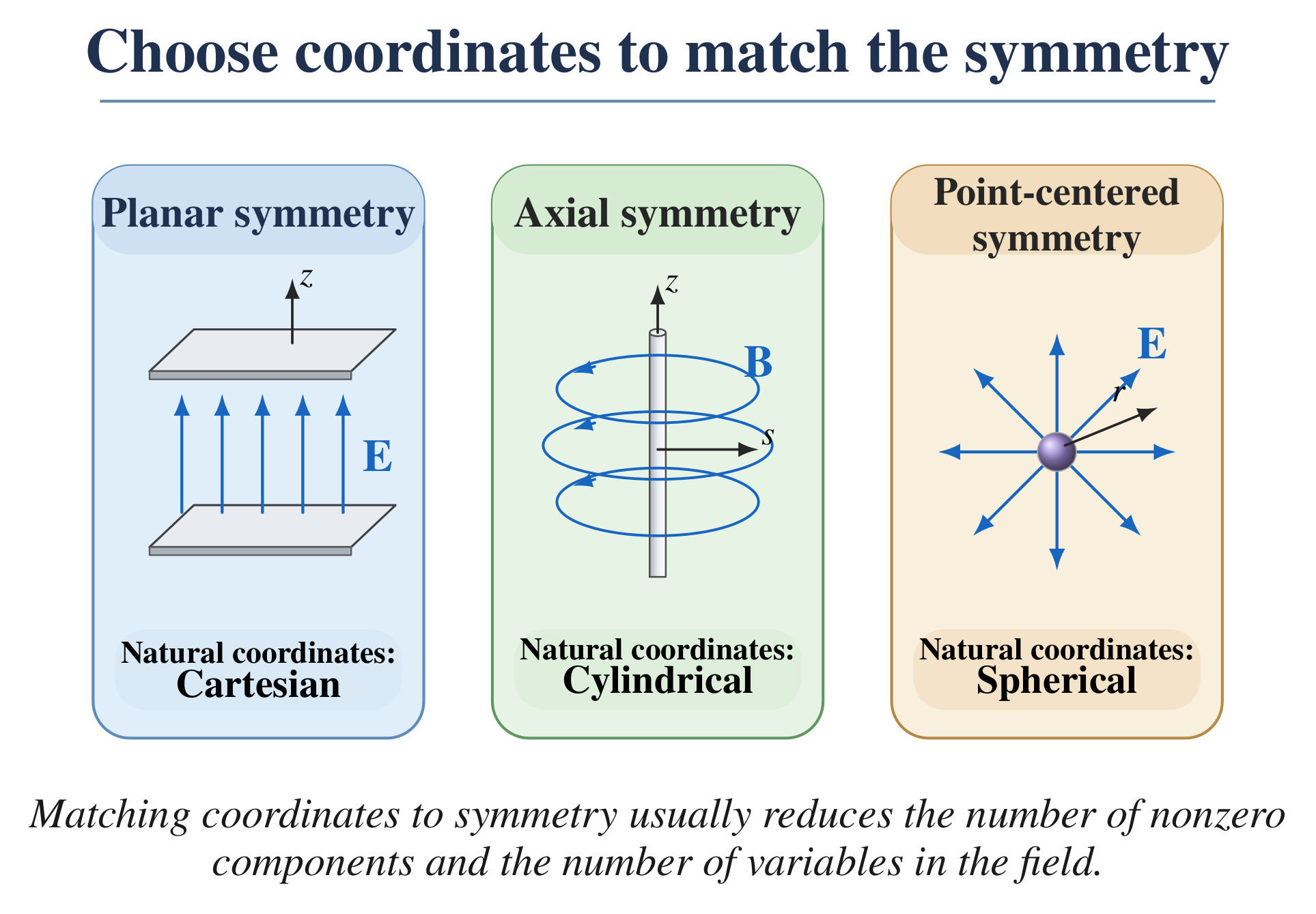
Figure 9. Coordinate choice should follow physical symmetry. Planar systems naturally suggest
Cartesian coordinates, axial systems cylindrical coordinates, and point-centered systems spherical
coordinates.
20 Worked example 1: components of a vector
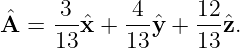
Let
Its magnitude is
| A | =  | (135)
|
| = 13. | (136) |
The unit vector in the direction of A is
If
then the scalar component of A along B is simply
21 Worked example 2: source-to-field displacement
Let the source point be
and the observation point be
Then
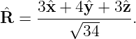
Its magnitude is
Therefore
This exact geometric construction appears in the field integral of a continuous charge
distribution.
22 Worked example 3: cylindrical basis at a specific point
Consider the point
Then
| s | = cos 60∘x + sin 60∘y | (146)
|
| =  x +  y, | (147) |
while
| ϕ | = − sin 60∘x + cos 60∘y | (148)
|
| = − x +  y. | (149) |
The basis is orthonormal:
At a different azimuth, the numerical Cartesian components of the cylindrical unit vectors change
even though the coordinate names remain s and ϕ.
23 Worked example 4: area of a spherical patch
At fixed radius r, consider a small patch spanning angular increments d𝜃 and dϕ.
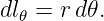
The meridional edge length is
The azimuthal edge length is
Therefore the patch area is
| da | = dl𝜃dlϕ | (153)
|
| = r2 sin 𝜃 d𝜃 dϕ. | (154) |
The corresponding outward vector area is
This is exactly the area element that will be used in spherical electric-flux calculations.
24 Bridge to the EDL laboratory series
The coordinate geometry developed here is directly measurable.
In EDL03, a potential map may be sampled on a rectangular grid:
The grid is a Cartesian coordinate description of the physical conducting sheet.
Later experiments may map magnetic fields around a wire or coil. Those measurements
often become clearer when replotted against cylindrical radius s or axial coordinate
z.
The important experimental lesson is that a coordinate system is part of the data model.
When recording a field measurement, one should specify
- where the sensor is located,
- what coordinate system describes that location,
- which direction the sensor measures,
- and which basis is used to report the measured components.
A Hall probe that reports one scalar channel is not directly measuring an entire vector B. It is
measuring a component of B along the probe’s sensitive axis.
Likewise, a potential probe measures a scalar V , not a vector field.
The distinction between field, component, coordinate, and instrument orientation is therefore
experimentally important, not merely mathematical bookkeeping.
25 Coordinate-choice workflow
For an electrodynamics problem:
- Identify the physical symmetry of the source and boundaries.
- Decide which coordinate surfaces naturally follow that geometry.
- Write the position vector in those coordinates.
- Derive or recall the basis vectors and scale factors.
- Construct the needed differential line, area, or volume element.
- Express the field components in the local basis.
- Only then perform the integral or differential operation.
This procedure reduces memorization and makes later formulas easier to reconstruct.
26 Common mistakes
- Treating a vector and its components as the same object.
- Forgetting that curvilinear basis vectors vary with position.
- Using dϕ as though it were a physical length rather than an angle.
- Omitting the factor s from cylindrical area or volume elements.
- Omitting r2 sin 𝜃 from spherical volume elements.
- Measuring spherical polar angle 𝜃 from the xy plane rather than from the +z axis
when using the Griffiths convention.
- Confusing the source coordinate r′ with the field coordinate r.
- Interpreting a coordinate singularity as automatically implying a physical singularity.
- Using a convenient coordinate system that does not respect the symmetry and then
hiding the physics under unnecessary algebra.
- Differentiating curvilinear vector components while silently treating the basis as
constant.
27 Practice exercises
- For A = 2x − 3y + 6z, find A and A.
- For A = x + 2y and B = 3x −y, compute A ⋅ B and the angle between them.
- For the same vectors, compute A × B and interpret its direction.
- Prove that A ⋅ (B × C) changes sign when any two vectors are exchanged.
- Starting from Equation (80), rederive s and ϕ.
- Show explicitly that s ⋅ϕ = 0.
- Starting from Equation (104), derive hr, h𝜃, and hϕ.
- Derive the cylindrical volume element from the product of physical edge lengths.
- Derive the spherical volume element from the three spherical scale factors.
- Explain why r sin 𝜃 dϕ becomes small near the poles even when dϕ is fixed.
- Write the Cartesian vector x in the cylindrical basis at arbitrary ϕ.
- Show that a radial cylindrical vector field F0s changes direction with ϕ even though
its radial component is constant.
- For a point charge at the origin, explain why spherical coordinates are symmetry
adapted before using any field equation.
- For an infinite straight wire along z, explain why ϕ is the natural magnetic-field
direction.
- Design a coordinate table for an EDL magnetic-field mapping experiment around a
straight current-carrying wire.
28 Companion files
Two compact reference files accompany this article in the PhysicsLibrary filebox.
These are intended as quick references while solving later ED and EDL problems.
29 Summary
A vector is a geometric object whose components depend on the chosen basis:
The dot product measures parallel alignment:
The cross product measures oriented perpendicular content:
For general orthogonal coordinates,
and
The volume element is
For cylindrical coordinates,
while for spherical coordinates,
These geometric results are the foundation from which ED03 will derive gradient, divergence, curl,
and the Laplacian rather than treating those operators as formulas to memorize.
References
References
[1] D. J. Griffiths, Introduction to Electrodynamics, 5th ed., Cambridge University Press,
2023.
[2] E. M. Purcell and D. J. Morin, Electricity and Magnetism, 3rd ed., Cambridge
University Press, 2013.
[3] H. M. Schey, Div, Grad, Curl, and All That, 4th ed., W. W. Norton, 2005.
[4] G. B. Arfken, H. J. Weber, and F. E. Harris, Mathematical Methods for Physicists,
7th ed., Academic Press, 2013.
[5] M. L. Boas, Mathematical Methods in the Physical Sciences, 3rd ed., Wiley, 2006.