Electromagnetic Waves, Antennas, and RF: Radiation from Time-Varying Currents and the
Hertzian Dipole
EM22 described electromagnetic energy guided along a transmission line. EM23 asks what happens
when a time-varying current distribution is allowed to launch fields into open space. The simplest
source that contains the essential physics is the Hertzian dipole: an ideal current element whose
length is much smaller than a wavelength. Although no physical antenna is literally infinitesimal,
this source is the basic building block for thin-wire antennas, radiation integrals, arrays, and
aperture methods [1, 2, 3, 4].
The central chain is
The most important physical distinction is that not every field surrounding an antenna is
a radiated field. Close to the source, electric and magnetic energy can be stored and
returned to the source each cycle. Far away, the surviving 1∕r terms carry net power
outward.
1 Time convention and propagation convention
Throughout this article, sinusoidal quantities use the phasor convention
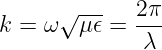
An outward traveling spherical wave therefore contains
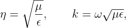
where
and, in a lossless medium,
In vacuum,
Writing the convention explicitly is important because reversing the sign convention for time
also reverses several i signs in the phasor formulas, while leaving all measurable powers
unchanged.
2 Why radiation must be retarded
Maxwell’s equations do not allow a change in source current to influence distant points
instantaneously. In a homogeneous medium with propagation speed
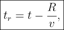
the field observed at position r depends on the source at the earlier retarded time
where
The time-domain magnetic vector potential is
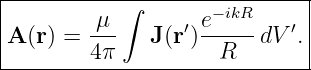
For sinusoidal steady state, retardation becomes a phase factor. The phasor vector potential
is
The factor 1∕R represents spherical amplitude spreading, while e−ikR records propagation phase.
This is the first mathematical appearance of the radiating 1∕r behavior that will dominate the far
field.
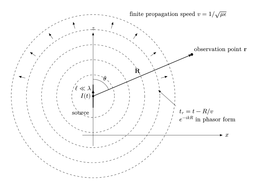
Figure. A time-varying current element at the source point influences an observation point
only after the propagation delay R∕v. In sinusoidal steady state, that delay becomes the
phase factor e−ikR.
3 The Hertzian current element
Place a very short current element of length ℓ at the origin and orient it along the z axis. Let its
current phasor be I0. The defining assumptions are
and
so the current element may be treated as spatially infinitesimal at the observation point.
Its current moment is
with units of ampere-meters. For an ideal Hertzian element the current is taken uniform over
ℓ.
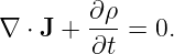
The associated end charges are not optional. Charge conservation requires
For harmonic time dependence,
Thus a time-varying short current element necessarily has a corresponding oscillating charge
distribution. The electric near field will contain the effect of those charges.
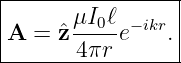
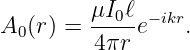
For the ideal element, the vector potential is
Define
Since
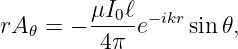
the spherical components are
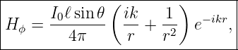
4 Deriving the magnetic field
The magnetic flux density is
For this axisymmetric source, only the ϕ component survives. The spherical-coordinate curl
gives
First,
so
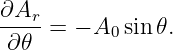
Also,
Therefore
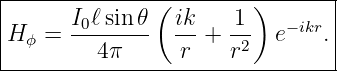
Since B = μH,
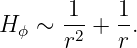
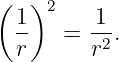
Two radial dependences already appear:
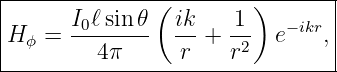
The 1∕r2 term is associated with the induction field; the 1∕r term survives into the radiation
zone.
5 Deriving the electric field
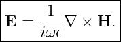
Outside the source region, J = 0, so the phasor Ampere-Maxwell law is
Hence
Because Hϕ is the only nonzero magnetic-field component,
and
Carrying out the derivatives and using
gives
and
Together with
these are the complete external fields of the ideal Hertzian current element under the stated phasor
convention.
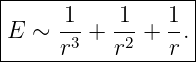
6 Three radial field scalings
The electric field contains three characteristic powers of distance:
They have different physical roles.
6.1 The 1∕r3 electrostatic-like term
The most rapidly decaying term appears in the electric field and is tied to the oscillating charge
separation. It resembles the static electric dipole field and dominates sufficiently close to the
source, while still outside the idealized source itself.
6.2 The 1∕r2 induction term
The 1∕r2 terms occur in both electric and magnetic fields. They are associated with induction and
with energy exchanged between the source and nearby fields. They decay faster than radiation and
therefore become progressively less important with distance.
6.3 The 1∕r radiation term
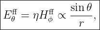
The 1∕r terms are special because their power density falls as
Multiplying by the area of a sphere,
produces a distance-independent total radiated power. This is exactly the geometric-spreading
behavior developed earlier in EM17.
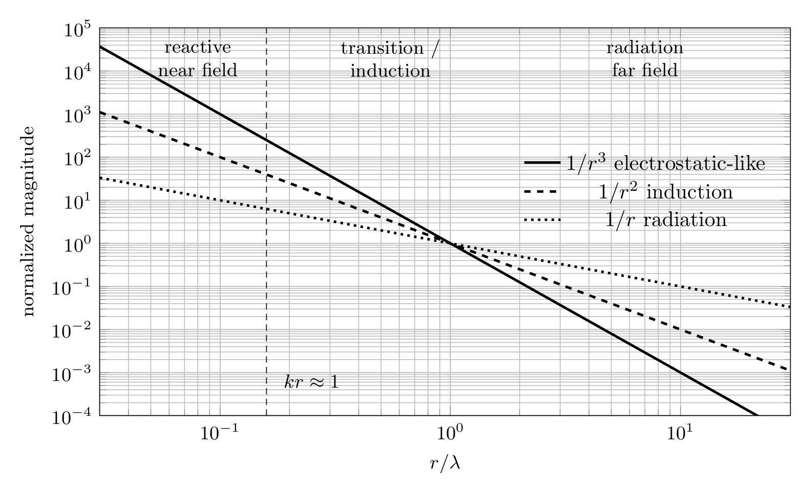
Figure. Radial scaling of the three field families. The labels “near”, “intermediate”, and
“far” describe dominant behavior, not infinitely sharp boundaries.
7 Near, intermediate, and far-field interpretation
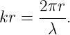
For the infinitesimal dipole, the dimensionless parameter controlling the hierarchy is
When
the 1∕r3 and 1∕r2 terms are important. This is the reactive near-field regime of the idealized
source.
When
no single radial power need dominate. This is the transition or induction region.
When
the 1∕r terms dominate. This is the far-field or radiation regime for the point-source
model.
For a real antenna of finite maximum dimension D, an additional far-field condition involving D is
required. A commonly used engineering criterion is
provided the observation point is also many wavelengths and many antenna dimensions away when
those constraints are relevant [1, 2]. The Hertzian element is idealized as D → 0, so the kr
hierarchy is the important one here.
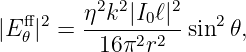
8 Far-field simplification
In the far field, retain only the 1∕r terms. Then
and
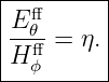
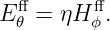
Therefore
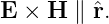
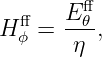
The far field has become locally plane-wave-like:
Also,
The source launches a spherical wave globally, but over a small patch of a sufficiently large sphere
the wavefront is approximately planar.
9 Why the near field is called reactive
The radial powers alone do not tell the whole story. Phase matters too. Near-field electric and
magnetic terms are not generally in the same phase. Energy is alternately stored in
the electric and magnetic fields and can flow back toward the source during part of a
cycle.
In contrast, the far-field terms share the same propagation phase and satisfy
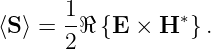
Their time-averaged Poynting vector is therefore outward and nonzero:
This is the physical distinction between merely having electromagnetic fields around a source and
actually radiating net energy to infinity.
10 Angular radiation pattern
The far-field electric amplitude contains the angular factor
Thus the field amplitude is zero on the dipole axis,
and maximum broadside to the dipole,
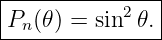
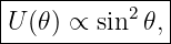
Because power is proportional to field amplitude squared, the normalized power pattern
is
The pattern is independent of azimuth ϕ. Rotating the two-dimensional figure-eight power cut
about the z axis produces the familiar doughnut-shaped three-dimensional radiation
pattern.
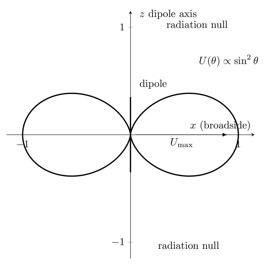
Figure. Normalized Hertzian-dipole power pattern in a plane containing the dipole axis. The
field is zero along the dipole and maximum broadside. Rotational symmetry about z gives
the three-dimensional doughnut pattern.
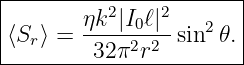
11 Far-field power density
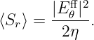
Using the far-field relation
the radial time-average Poynting vector is
Since
we obtain
The 1∕r2 dependence of power density is now explicit.
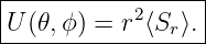
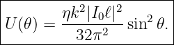
12 Radiation intensity
A useful distance-independent quantity is the radiation intensity
For the Hertzian dipole,
Its units are watts per steradian. Radiation intensity removes the trivial spherical-spreading factor
and leaves only the angular distribution of radiated power.
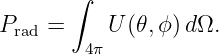
13 Total radiated power
The total power passing through a large sphere is
Using
we have
| Prad | =  ∫
02πdϕ∫
0π sin 3𝜃 d𝜃. ∫
02πdϕ∫
0π sin 3𝜃 d𝜃. | (66) |
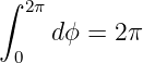
The angular integrals are
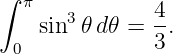
and
Therefore
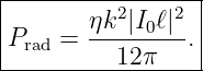
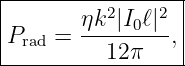
In free space, use
and
to obtain
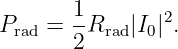
Here I0 is the peak phasor current amplitude; the factor 1∕2 associated with time averaging has
already been included.
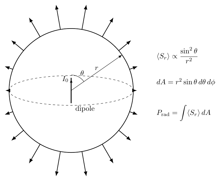
Figure. Total radiated power is obtained by integrating the outward far-field Poynting flux
over any sufficiently large sphere. The local flux varies as sin 2𝜃∕r2, while the area element
grows as r2 sin 𝜃 d𝜃 dϕ.
14 Radiation resistance
It is convenient to represent the radiated power by an equivalent resistance defined
through
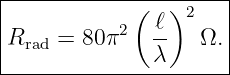
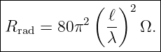
Comparing with the free-space radiated-power expression gives
This is not an ohmic resistor. It is a circuit representation of real power carried away by
electromagnetic radiation.
A terminology warning is important. The formula above is for the ideal Hertzian or infinitesimal
dipole with uniform current I0 over length ℓ. A physically short center-fed dipole has an
approximately triangular current distribution and a different radiation-resistance coefficient. The
two models should not be mixed.
15 Directivity of the Hertzian dipole
Although antenna gain will be developed systematically in EM24, the radiation pattern already
lets us calculate directivity.
The maximum radiation intensity occurs at
so
The average radiation intensity over all directions is
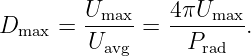
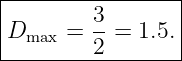
Therefore the maximum directivity is
Substitution gives
In decibels relative to isotropic,
This is directivity, not yet gain. Gain will require radiation efficiency as well as angular
concentration.
16 Worked numerical example
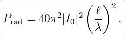
Consider an ideal Hertzian element in free space at
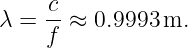
The wavelength is
Let
and let the peak current amplitude be
The radiation resistance is
| Rrad | = 80π2 2 2 | (85)
|
| ≈ 0.3158 Ω. | (86) |
Thus
Now observe the antenna broadside at
The far-field electric amplitude is
The magnetic amplitude is
The average local power density is
The result is small locally because the radiated energy has spread over a large spherical area, but
integration over all directions recovers the same 0.1579 W total radiated power.
17 General far-field current-distribution form
The Hertzian element is a building block for arbitrary antennas. For a localized current
distribution observed far away, write
When
we use the far-zone approximations
and
Therefore
The vector potential becomes
This expression contains one of the central ideas of antenna theory: radiation in a given direction is
a coherent sum of contributions from the entire current distribution, each weighted by its
relative propagation phase. Antenna patterns and phased arrays ultimately grow from this
phase-summation principle.
18 What changes between near field and far field
Several properties emerge together in the far zone:
- the 1∕r field terms dominate;
- the radial electric component becomes negligible;
- E, H, and r become mutually perpendicular;
- the field ratio approaches the medium impedance η;
- electric and magnetic far fields are in phase for a lossless medium;
- the average Poynting vector is directed radially outward;
- angular pattern becomes independent of distance;
- power density falls as 1∕r2.
These are precisely the properties needed to connect Maxwell’s equations to practical antenna
quantities such as radiation intensity, directivity, gain, effective aperture, EIRP, and eventually the
Friis transmission equation.
19 Common mistakes
- Calling every 1∕r2 quantity a near field. Far-field power density falls as 1∕r2 even
though the far-field field amplitudes fall as 1∕r.
- Assuming the near field carries no instantaneous power. Energy can flow locally
in either direction. The distinction is that reactive energy is returned rather than
producing a distance-independent net radiated power.
- Dropping Er everywhere. The radial electric field is negligible in the far zone, not
in the general Hertzian-dipole solution.
- Using a far-field formula at kr ≪ 1. The discarded 1∕r2 and 1∕r3 terms can then
dominate.
- Confusing field pattern with power pattern. The Hertzian field amplitude is
proportional to sin 𝜃; the power pattern is proportional to sin 2𝜃.
- Mixing peak and RMS current conventions. Here I0 is a peak phasor amplitude,
so P = (1∕2)R|I0|2.
- Confusing Hertzian and physically short dipoles. Their current distributions,
and therefore their radiation-resistance coefficients, differ.
20 What EM23 adds to the series
EM16–EM21 established electromagnetic waves, energy flow, propagation, polarization, and
boundary behavior. EM22 showed how those waves can be guided on transmission lines. EM23 now
makes the transition from guided waves to radiation from sources.
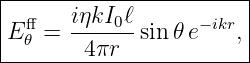
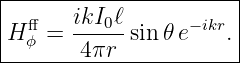
The key field results for the ideal z-directed Hertzian element are
and
In the radiation zone,
which leads to
and in free space
The next article can build directly on these results to define radiation intensity, beam
solid angle, directivity, radiation efficiency, antenna gain, EIRP, and effective aperture
systematically.
References
[1] C. A. Balanis, Antenna Theory: Analysis and Design, 4th ed., Wiley, 2016.
[2] W. L. Stutzman and G. A. Thiele, Antenna Theory and Design, 3rd ed., Wiley,
2012.
[3] D. J. Griffiths, Introduction to Electrodynamics, 4th ed., Cambridge University Press,
2017.
[4] J. D. Jackson, Classical Electrodynamics, 3rd ed., Wiley, 1999.
[5] S. Ramo, J. R. Whinnery, and T. Van Duzer, Fields and Waves in Communication
Electronics, 3rd ed., Wiley, 1994.
[6] F. T. Ulaby and U. Ravaioli, Fundamentals of Applied Electromagnetics, 7th ed.,
Pearson, 2015.















![[ ]
1- ∂-(rA𝜃) ∂Ar-
(∇ × A )ϕ = r ∂r − ∂𝜃 .](https://images.physicslibrary.org/cache/objects/1449/make4ht/ElectromagneticWavesAntennasAndRFRadiationFromTimeVaryingCurrentsAndTheHertzianDipole21x.png)