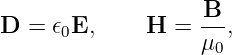
Electromagnetic Waves, Antennas, and RF: Electromagnetic Energy, the Poynting Vector, and
Intensity
EM16 showed that Maxwell’s equations support electromagnetic waves in vacuum. A wave
equation tells us how a disturbance propagates, but it does not yet answer another fundamental
physical question:
The answer is encoded directly in Maxwell’s equations. Electric and magnetic fields possess energy
density, and the flow of electromagnetic energy is described by the Poynting vector. Combining
those ideas gives a local conservation law for electromagnetic energy called Poynting’s
theorem.
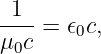
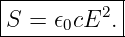
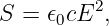
For a plane electromagnetic wave in vacuum, the result becomes especially simple:
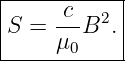
and, because E = cB for a vacuum plane wave,
These relations connect the field picture of Maxwell’s equations to measurable power, intensity,
antenna radiation, and eventually RF link budgets [1, 2, 3, 4, 5].
1 Energy stored in an electric field
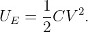
The electrostatic energy density can be motivated from a parallel-plate capacitor. The energy
stored in a capacitor is
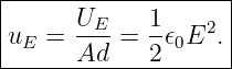
For a vacuum parallel-plate capacitor with plate area A and spacing d,
Neglecting fringing, the Electric Field between the plates is approximately uniform:
Therefore
| UE | =   V 2 V 2 | (8)
|
| =  𝜖0 𝜖0 (Ed)2 (Ed)2 | (9)
|
| =  𝜖0E2Ad. 𝜖0E2Ad. | (10) |
The volume occupied by the approximately uniform field is
Hence the energy per unit volume is
This result suggests a useful physical viewpoint: the capacitor stores energy in the electric field
distributed through the space between the plates.
2 Energy stored in a magnetic field
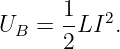
A similar argument can be made using an ideal long solenoid. The magnetic energy stored in an
inductor is
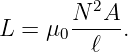
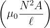
For a long vacuum solenoid of length ℓ, cross-sectional area A, and N turns,
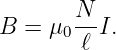
The magnetic field inside is approximately
Solve for the current:
Substitute into the inductive energy:
Since Aℓ is the field-filled volume,
Thus a magnetic field also stores energy locally.
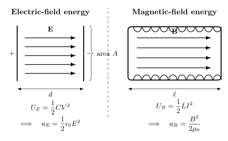
Figure. The familiar lumped-element energies UE = CV 2∕2 and U
B = LI2∕2 can be
rewritten as energy distributed through the electric and magnetic fields. In vacuum the
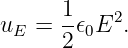
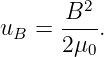
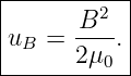
corresponding field-energy densities are uE = 𝜖0E2∕2 and u
B = B2∕(2μ
0).
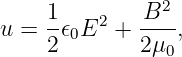
3 Total electromagnetic energy density in vacuum
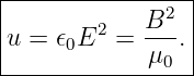
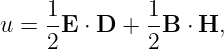
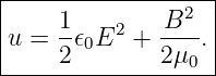
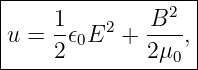
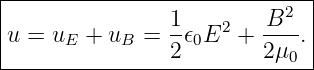
When both fields are present, the total electromagnetic energy density is
Here u has units of energy per volume:
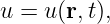
For fields that vary with position and time,
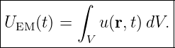
and the total field energy inside a volume V is
The next question is not how much energy is present, but how that energy moves from one place to
another.
4 A conservation law must contain an energy flux
For any conserved quantity, a local conservation equation has the general form
For electromagnetic energy, the accumulation term will be
The energy-flux term must have units of power per area,
because its surface integral must give power. Maxwell’s equations tell us exactly what this flux
vector is.
5 Deriving Poynting’s theorem from Maxwell’s equations
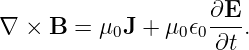
Begin with the Ampere–Maxwell law in vacuum with a possibly nonzero conduction current
density J:
Take the dot product with E and divide by μ0:
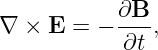
Now take Faraday’s law,
and dot it with B∕μ0:
The Vector Identity that connects the two curl terms is
Substituting the two Maxwell Equations into this identity gives
 ∇⋅ (E × B) ∇⋅ (E × B) | = − B ⋅ B ⋅ − J ⋅ E − 𝜖0E ⋅ − J ⋅ E − 𝜖0E ⋅ . . | (32) |
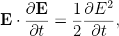
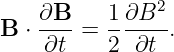
Now use
and
Therefore
 ∇⋅ (E × B) ∇⋅ (E × B) | = − 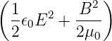 − J ⋅ E. − J ⋅ E. | (35) |
Move every term to the left:
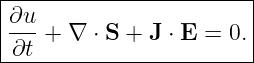
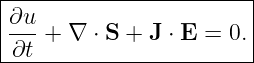
This is the differential form of Poynting’s theorem.
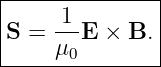
6 Definition of the Poynting vector
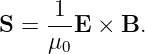
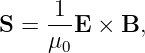
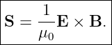
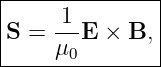
The energy-flux vector appearing naturally in the derivation is
The Poynting vector points in the direction of electromagnetic energy flow. Its SI units
are
With this definition and the energy density u, Poynting’s theorem becomes
Each term has units of power per volume:
7 What does J ⋅ E mean?
The electromagnetic force density on charges includes the electric contribution
For a small collection of moving charge, power is force dotted with velocity. In continuum form,
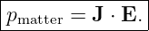
the electrical power delivered to matter per unit volume is
If
the electromagnetic field is doing positive work on matter. Field energy is being converted into
mechanical energy, thermal energy, chemical energy, or some other material form.
For an ordinary resistor with Ohm’s law
we obtain
which is the local form of Joule heating.
If J ⋅ E < 0, matter is transferring energy back into the electromagnetic field, as occurs in
generators or radiating sources during appropriate parts of their operation.
8 Integral form of Poynting’s theorem
Integrate the local conservation equation over a fixed volume V :
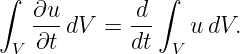
For a fixed integration volume,
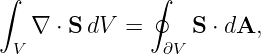
Use the divergence theorem on the flux term:
where dA points outward. Therefore
This equation has a direct bookkeeping interpretation:
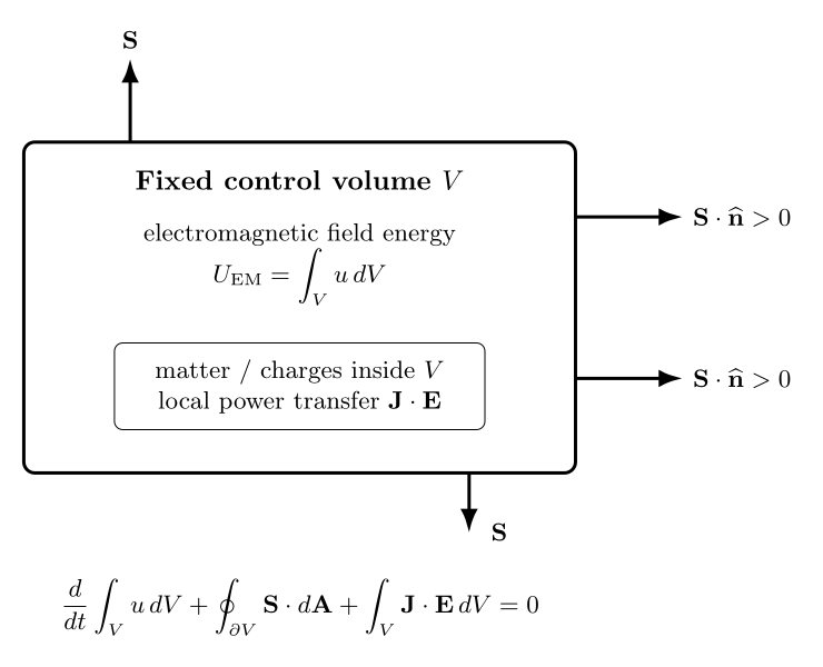
Figure. Poynting’s theorem is an energy balance for a fixed control volume.
Electromagnetic energy can accumulate inside the volume, flow through the boundary
through S, or be transferred to matter through J ⋅ E.
9 Example 1: steady power absorbed by a resistor
Suppose a resistor is enclosed by a fixed surface. In steady operation the electromagnetic energy
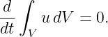
stored inside the chosen volume is not changing appreciably, so
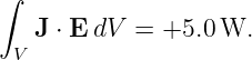
If the resistor absorbs 5.0 W,
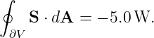
Poynting’s theorem therefore requires
The negative outward flux means that 5.0 W of electromagnetic power flows into the control
volume and is delivered to the resistor.
This is a useful conceptual correction to the informal idea that electrical energy simply “travels
inside the wire.” In the field description, electromagnetic energy flows through the surrounding
fields and is transferred into matter where J ⋅ E is positive.
10 Poynting vector for a vacuum plane wave
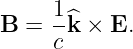
EM16 established that a plane wave propagating in direction k satisfies
Therefore
and the electric field, magnetic field, and propagation direction are mutually perpendicular.
The Poynting vector is
Because E ⊥ B,
Use B = E∕c:
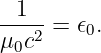
Since
we may also write
Equivalently, using E = cB,
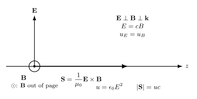
Figure. For a vacuum plane wave, E, B, and the energy-flow direction are mutually
perpendicular. The Poynting vector points in the same direction as wave propagation.
11 Electric and magnetic energies are equal in a vacuum plane wave
The electric energy density is
The magnetic energy density is
For a plane wave,
Thus
But
Therefore
The total energy density is consequently
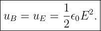
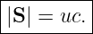
Comparing this with the Poynting magnitude,
gives
This has an intuitive interpretation: a plane wave with energy density u transports that energy at
speed c.
12 Sinusoidal waves: instantaneous energy flow
Consider a linearly polarized harmonic wave propagating in +z:
with
The instantaneous Poynting vector is
| S | =  E × B E × B | (75)
|
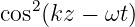
| =  cos 2(kz − ωt)z. cos 2(kz − ωt)z. | (76) |
Using B0 = E0∕c,
Because cos 2 is never negative, the energy flux remains in the +z direction even while the field
components themselves reverse sign every half cycle.
13 Intensity is the time-averaged Poynting flux
For rapidly oscillating electromagnetic waves, instruments often respond to energy averaged over
many periods rather than to the instantaneous carrier oscillation. The time average
of
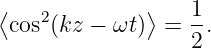
over one period is
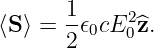
Therefore the average Poynting vector is
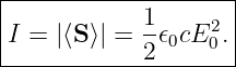
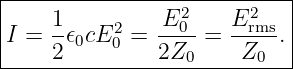
The intensity of the plane wave is the magnitude of this time-averaged energy flux:
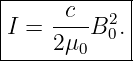
Using the magnetic-field amplitude,
The distinction is important:
- S(r,t) is the instantaneous electromagnetic power-flow density;
- ⟨S⟩ is its time average;
- intensity I commonly denotes the magnitude of the time-averaged Poynting vector for
a periodic traveling wave.
14 RMS fields and the vacuum impedance
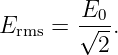
For a sinusoidal electric field,
Therefore
| I | =  𝜖0cE02 𝜖0cE02 | (84)
|
| = 𝜖0cErms2. | (85) |
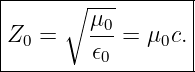
Define the vacuum wave impedance
Numerically,
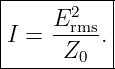
Since
we obtain the useful RF relation
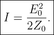
In terms of peak electric-field amplitude,
These are electromagnetic analogues of familiar power relations in circuit theory. The impedance
Z0 links electric and magnetic field amplitudes in a traveling wave.
15 Example 2: intensity of a 1 V/m plane wave
Suppose a sinusoidal vacuum plane wave has peak electric-field amplitude
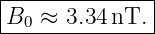
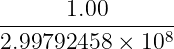
Its magnetic-field amplitude is
| B0 | =  | (92)
|
| =  | (93)
|
| = 3.34 × 10⁻⁹ T. | (94) |
Thus
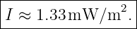
The average intensity is
| I | =  𝜖0cE02 𝜖0cE02 | (96)
|
| ≈ 1.33 × 10⁻³ W/m2. | (97) |
Therefore
A field amplitude that sounds modest in volts per meter can therefore be translated directly into
an energy-flow density.
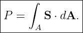
16 Power crossing an arbitrary surface
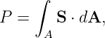
If an electromagnetic field crosses a surface A, the instantaneous power through that surface
is
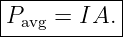
For a uniform plane wave normally incident on a flat area A,
For a sinusoidal wave, the average power is
If the wave arrives at an angle 𝜃 relative to the surface normal,
The factor A cos 𝜃 is the projected area presented to the power flow.
17 Spherical spreading and the inverse-square law
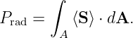
Now consider an ideal isotropic source radiating total time-averaged power Prad uniformly in
all directions. Far enough from the source, imagine a sphere of radius r surrounding
it.
Conservation of energy requires the same total radiated power to cross every such sphere:
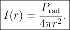
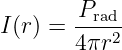
For an isotropic source the intensity is uniform over the sphere, so
Therefore
This is the electromagnetic inverse-square law for power density in lossless free-space spherical
spreading.
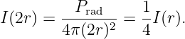
If the radius doubles,
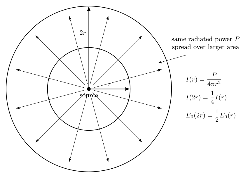
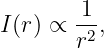
Figure. In lossless spherical spreading the same radiated power crosses spheres whose area
grows as 4πr2. Intensity therefore falls as 1∕r2. Because intensity is proportional to field
amplitude squared, the field amplitudes fall as 1∕r.
18 Why field amplitude falls as 1∕r
The inverse-square law describes power density. It does not say that the electric-field amplitude
falls as 1∕r2.
For a plane-wave-like far field,
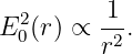
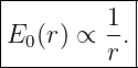
If spherical spreading gives
then
Taking the positive square root of the amplitude relation gives
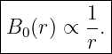
Because B0 = E0∕c,
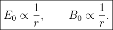
This is the key connection between power spreading and amplitude spreading:
19 Deriving the far-field electric amplitude of an isotropic radiator
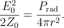
Combine
with
Then
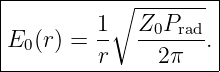
Solve for the peak electric-field amplitude:
Therefore
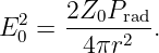
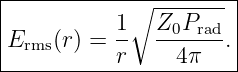
For the RMS field,
The 1∕r dependence is therefore not an independent empirical rule. It follows from conservation of
radiated power plus the fact that electromagnetic intensity is proportional to the square of field
amplitude.
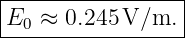
20 Example 3: a 10 W isotropic radiator at 100 m
Let
The intensity is
| I | =  | (120)
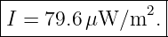
|
| = 7.96 × 10⁻⁵ W/m2. | (121) |
Thus
The RMS electric field is
| Erms | =  | (123)
|
| =  | (124)
|
| ≈ 0.173 V/m. | (125) |
The peak amplitude is
Therefore
The corresponding magnetic amplitude is
If the distance is doubled to 200 m, intensity falls by a factor of four while E0 and B0 each fall by a
factor of two.
21 Directional radiation and gain
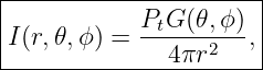
Real antennas are generally not isotropic. They redistribute radiated power with direction. In the
far field, the power density in a particular direction is commonly written
where Pt is transmitter power delivered to the radiating system under the convention being used
and G(𝜃,ϕ) is antenna gain in the specified direction.
The product
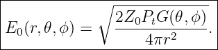
is the quantity that leads to effective isotropic radiated power in a chosen direction. Combining the
gain form with
gives
This relation is a direct bridge from Maxwell’s field quantities to the power-density language used
in antenna and RF engineering.
22 The far-field qualification matters
The simple relations
are traveling-wave or radiation-zone relations. Close to an antenna, reactive electric and magnetic
fields can store and return energy rather than carry it irreversibly outward.
In such a near-field region:
- E and B need not have the simple plane-wave amplitude ratio;
- the instantaneous Poynting vector can have complicated spatial structure;
- some field energy can oscillate back and forth near the source;
- a simple 1∕r2 intensity law need not describe every field component.
Far from a localized radiator, the radiative terms dominate and the field approaches the
transverse-wave behavior developed in EM16 and this article.
23 A useful distinction: energy density, flux, intensity, and power
These quantities are related but should not be confused.
Energy density
with units J/m3.
Instantaneous Poynting vector
with units W/m2.
Intensity for a periodic traveling wave
also with units W/m2.
Power through a surface
with units W.
The progression is therefore
24 Extension to simple material media
In a simple linear, nondispersive medium, the energy density is commonly written
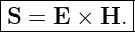
and the Poynting vector is
In vacuum,
so these reduce to the formulas derived above.
Caution is required for strongly dispersive, lossy, nonlinear, or anisotropic media because the
relation between stored field energy and the constitutive response can require additional terms or
more careful definitions. The vacuum result remains the cleanest starting point.
25 Common mistakes
- Confusing energy density u in J/m3 with intensity I in W/m2.
- Forgetting that the Poynting vector is a vector: its direction matters as much as its
magnitude.
- Using S = EB∕μ0 without first checking that E and B are perpendicular.
- Using E = cB for arbitrary static or near-field configurations. This is a plane-wave or
radiation-zone relation in vacuum.
- Forgetting the factor 1∕2 when converting sinusoidal peak amplitudes to time-averaged
intensity.
- Mixing peak and RMS field amplitudes. For a sinusoid, Erms = E0∕
 .
.
- Assuming that field amplitude obeys a 1∕r2 law. In spherical radiation, intensity scales
as 1∕r2 while field amplitudes scale as 1∕r.
- Applying I = P∕(4πr2) to a directional antenna without including its radiation pattern
or gain.
- Applying far-field inverse-square relations inside a reactive near field.
- Misreading the sign of J ⋅ E. Positive J ⋅ E means electromagnetic energy is being
delivered to matter.
26 What EM17 adds to the series
EM16 established that Maxwell’s equations support waves. EM17 adds the energy interpretation of
those waves.
The vacuum electromagnetic energy density is
The electromagnetic energy-flux vector is
Maxwell’s equations imply the conservation law
For a sinusoidal plane wave in vacuum,
Finally, conservation of radiated power over an expanding sphere gives
while the electromagnetic field amplitudes scale as
These results form the energy bridge from Maxwell’s equations to antennas, RF propagation,
received power, and link-budget calculations.
References
[1] David J. Griffiths, Introduction to Electrodynamics, 4th ed., Cambridge University
Press, 2017.
[2] Edward M. Purcell and David J. Morin, Electricity and Magnetism, 3rd ed.,
Cambridge University Press, 2013.
[3] Samuel J. Ling, Jeff Sanny, and William Moebs, University Physics, Volume
2, OpenStax, 2016, sections on electromagnetic energy, Poynting’s theorem, and
electromagnetic waves.
[4] Richard P. Feynman, Robert B. Leighton, and Matthew Sands, The Feynman Lectures
on Physics, Volume II, Addison-Wesley, 1964, chapters on electromagnetic energy and
energy flow.
[5] Massachusetts Institute of Technology, 8.02 Physics II: Electricity and Magnetism,
MIT OpenCourseWare, materials on Maxwell’s equations, electromagnetic waves, energy
density, and the Poynting vector.









![3
[u] = J/m .](https://images.physicslibrary.org/cache/objects/1241/make4ht/ElectromagneticWavesElectromagneticEnergyThePoyntingVectorAndIntensity24x.png)







![[S] = W/m2.](https://images.physicslibrary.org/cache/objects/1241/make4ht/ElectromagneticWavesElectromagneticEnergyThePoyntingVectorAndIntensity46x.png)