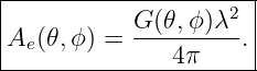
Electromagnetic Waves, Antennas, and RF: Antenna Directivity, Radiation Efficiency, Gain, EIRP,
and Effective Aperture
EM23 derived the radiation field of a Hertzian dipole and showed that a localized time-varying
current distribution launches electromagnetic power into different directions with different
strengths. EM24 now turns that radiation pattern into the antenna quantities used throughout RF
engineering: directivity, radiation efficiency, gain, equivalent isotropically radiated power, and
effective aperture. The central objective is to connect every one of these quantities back to
electromagnetic power flow rather than treat them as isolated link-budget definitions
[1, 2, 3, 4].
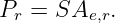
The central chain is
The final result,
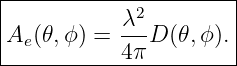
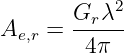
will be derived first for the Hertzian dipole and then generalized using antenna reciprocity. This
relation is the missing bridge between a transmitting antenna’s directional gain and a receiving
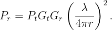
antenna’s ability to intercept power. EM25 will use it to derive the Friis transmission equation and
free-space path loss.
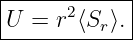
1 Radiation intensity revisited
In the far field, the time-average Poynting vector is approximately radial,
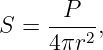
Because a radiated field amplitude decreases as 1∕r, its power density decreases as 1∕r2. It is
therefore useful to remove this purely geometric spreading by defining the radiation
intensity
Its units are watts per steradian,
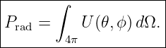
The total radiated power is obtained by integrating over solid angle:
With spherical coordinates,
so
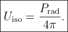
An isotropic radiator is the reference source that distributes the same power equally into every
direction. Its radiation intensity is therefore

Figure. Directivity compares the actual radiation intensity in a selected direction with the
intensity that an isotropic radiator would produce if it radiated the same total power.
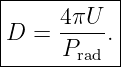
2 Directivity
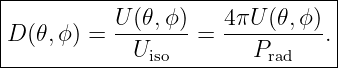
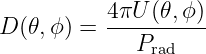
The directional directivity is defined as
Directivity is dimensionless. It measures only how the radiated power is distributed in angle. It
does not yet penalize Conductor loss, dielectric loss, or other dissipative mechanisms inside the
antenna.
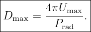
The maximum directivity is
Antenna values are often expressed logarithmically relative to an isotropic radiator:
The suffix dBi means decibels relative to an ideal isotropic radiator.
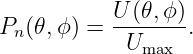
3 Beam solid angle
Let the normalized power pattern be
Then
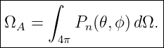
Define the beam solid angle
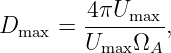
Substituting into the maximum-directivity definition gives
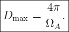
so
This expression captures the physical idea of directivity: a pattern concentrated into a smaller solid
angle has a larger peak directivity.
4 Example: Hertzian-dipole directivity
EM23 found the normalized power pattern of a Hertzian dipole,
Therefore
| ΩA | = ∫
02π ∫
0π sin 2𝜃 sin 𝜃 d𝜃 dϕ | (19)
|
| = 2π ∫
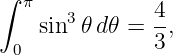
0π sin 3𝜃 d𝜃. | (20) |
Using
we obtain
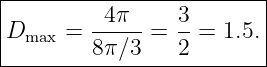
Hence
In logarithmic form,
This value describes angular concentration only. An ideal Hertzian dipole is being treated as
lossless here.
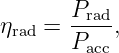
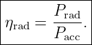
5 Radiation efficiency
A real antenna may accept power at its terminals without radiating all of it. Let
be the time-average power accepted by the antenna terminals. This power is divided into radiated
power and dissipative loss,
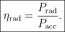
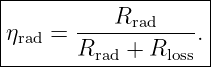
The radiation efficiency is
Therefore
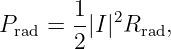
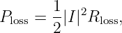
For a simple equivalent circuit containing radiation resistance Rrad and loss resistance Rloss in
series,
so
This makes the difficulty of electrically small antennas visible. If Rrad becomes very small while
conductor and matching-network losses remain finite, the radiation efficiency can fall
sharply.
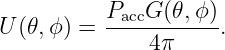
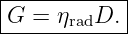
6 Gain
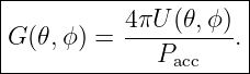
Directivity normalizes radiation intensity by the power actually radiated. Gain instead normalizes
by the power accepted at the antenna terminals:
Using
and
we obtain
Thus directivity answers
while gain answers
Maximum gain is usually quoted in dBi:
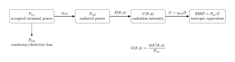
Figure. Accepted terminal power is first reduced by dissipative antenna losses; the
remaining radiated power is then distributed directionally. Gain combines radiation
efficiency and directivity.
7 Mismatch and realized gain
The gain defined above uses power accepted by the antenna. If a source delivers incident power
toward an antenna port with reflection coefficient ΓA, the accepted fraction is
A useful quantity that includes this mismatch is the realized gain,
The distinction matters in practical link budgets:
Cable and feed losses before the antenna are normally accounted for separately unless they have
explicitly been included in the quoted system gain.
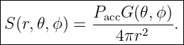
8 Equivalent isotropically radiated power
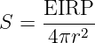
Suppose an antenna accepts transmit power Pacc and has directional gain G(𝜃,ϕ). In its far
field,
Therefore the power density at range r is
The product
is the equivalent isotropically radiated power: the power an isotropic radiator would need in order
to produce the same far-field power density in that direction.
In logarithmic units,
If cable, filter, or connector loss Lfeed,dB lies between the transmitter and antenna, a common
system form is
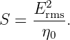
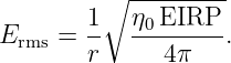
For free-space propagation, the corresponding RMS electric-field magnitude is
Substituting
gives
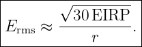
Because
we obtain the useful free-space relation
Here EIRP is in watts, r in meters, and the result is in volts per meter.
9 Example: efficiency, gain, and EIRP
Consider an antenna with maximum directivity
and radiation efficiency
The maximum gain is
In dBi,
If the antenna accepts
then
This does not mean the antenna radiates 150 W of total power. The total radiated power is
only
The larger EIRP expresses directional concentration relative to an isotropic radiator.
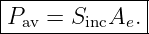
10 Receiving antennas and effective aperture
Now reverse the problem. Let a plane wave with time-average power density
arrive at a receiving antenna from some direction. The antenna produces electrical power at its
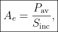
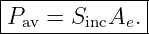
terminals. For conjugate load matching and matched polarization, define the effective aperture
by
where Pav is the maximum available receive power.
Therefore
Although Ae has units of square meters, it is not necessarily the literal geometric shadow of the
antenna. A wire antenna may have negligible physical cross-sectional area yet possess a finite
effective aperture.
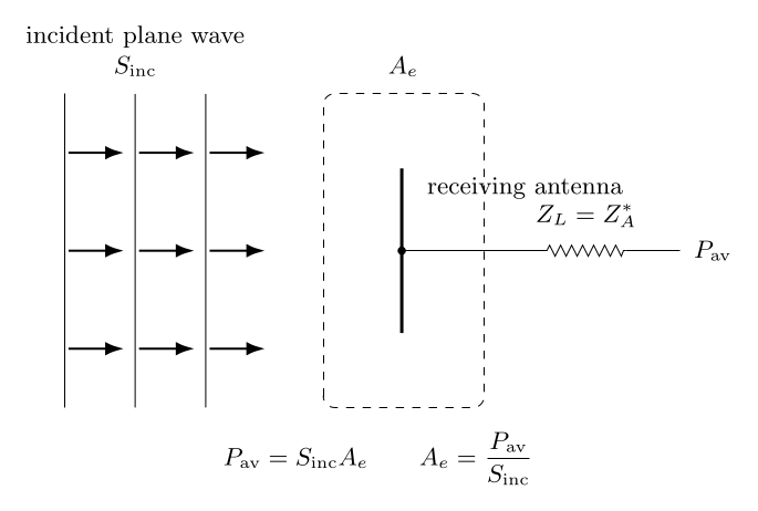
Figure. Effective aperture converts incident electromagnetic power density into maximum
available terminal power. It is an electromagnetic receiving property, not simply the
antenna’s physical silhouette.
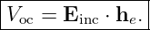
11 The receive effective length
A receiving antenna can also be characterized by an effective length vector he. The open-circuit
terminal voltage is
For an ideal Hertzian dipole oriented parallel to the incident Electric Field at broadside,
so
Here E is the peak phasor magnitude, consistent with the phasor convention used in
EM23.
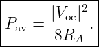
If the antenna input impedance is purely resistive at Resonance,
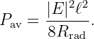
and a conjugate matched load is connected, the load voltage amplitude is V oc∕2. The maximum
time-average delivered power is therefore
For an ideal lossless Hertzian dipole,
12 Deriving the effective aperture of a Hertzian dipole
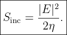
The time-average power density of a plane wave in a lossless medium is
For the broadside, polarization-matched Hertzian dipole,
so
Hence
| Ae | =  | (71)
|
| = 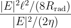 | (72)
|
| =  . . | (73) |
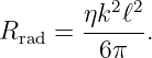
EM23 derived the radiation resistance of the ideal current element in a lossless medium,
Substituting gives
Using
we obtain
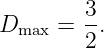
But EM23 also found
Therefore
Thus the transmit directivity and receive effective aperture satisfy
for the ideal lossless Hertzian dipole.
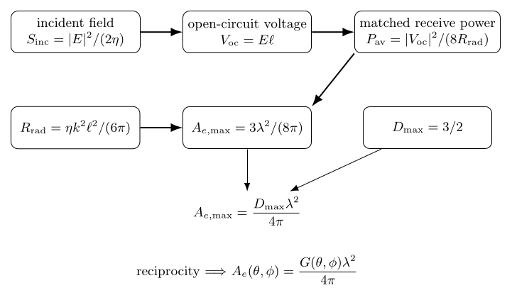
Figure. For the Hertzian dipole, receive voltage and maximum available power lead directly
to Ae = 3λ2∕(8π). The transmit result D
max = 3∕2 then reveals the general λ2∕(4π)
normalization.
13 From the Hertzian dipole to the general aperture-gain theorem
For a linear reciprocal antenna, the Lorentz reciprocity theorem implies that the angular and
polarization properties used to transmit a field are the same properties that govern reception from
that direction [1, 2]. Therefore the directional receive aperture has the same normalized angular
dependence as the transmit gain.
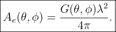
For a lossless antenna, the Hertzian result generalizes to
If the antenna has radiation efficiency less than unity, only the fraction ηrad of the receive-mode
electromagnetic power associated with the antenna mode is available at the terminals.
Since
the general matched-polarization, conjugate-match relation becomes
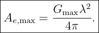
At the direction of maximum gain,
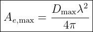
This is one of the most important antenna relations in RF engineering.
14 Physical meaning of the λ2 factor
At fixed dimensionless gain,
Thus the same 0 dBi receiving antenna has a larger effective area at a lower frequency. This does
not violate energy conservation. Gain is a dimensionless statement about angular coupling to a
propagating spatial mode, while the transverse spatial scale of that mode grows with
wavelength.
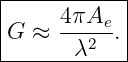
Conversely, for a fixed physical aperture whose effective area is nearly fixed, the gain rises
approximately as
This is why a fixed-size dish antenna becomes more directive as frequency increases.
15 Example: effective aperture at GPS L1
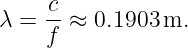
For the GPS L1 carrier,
The free-space wavelength is approximately
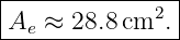
For an antenna with
its maximum effective aperture is
| Ae | =  | (91)
|
| ≈ 2.88 × 10⁻³ m2. | (92) |
Therefore
The effective electromagnetic collection area is much more meaningful than the visible
cross-sectional area of a small GNSS antenna.
16 Example: Hertzian-dipole effective aperture
At
the wavelength is approximately
For the ideal Hertzian dipole,
Hence
| Ae,max | = 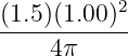 | (97)
|
| ≈ 0.119 m2. | (98) |
So an electrically tiny ideal current element can possess an effective aperture of order a tenth of a
square meter at a one-meter wavelength. Effective aperture is a coupling area, not a literal metal
area.
17 Polarization mismatch
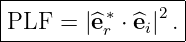
EM19 showed that a receiving antenna need not be polarization matched to the incident wave. If
the normalized incident polarization vector is ei and the receive polarization vector is er, the
polarization loss factor is
The available receive power becomes
For two linearly polarized antennas misaligned by angle ψ,
Thus effective aperture should normally be interpreted as the aperture under matched-polarization
conditions unless a polarization factor is stated separately.
18 Physical aperture and aperture efficiency
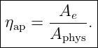
For aperture antennas such as horns, reflectors, or planar arrays, it is useful to compare effective
aperture with physical aperture Aphys. Define the aperture efficiency
Then
Combining this with the aperture-gain theorem gives
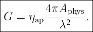
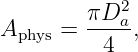
For a circular aperture of diameter Da,
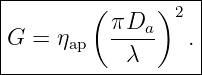
so
This is the standard scaling behind parabolic-dish antenna gain. The aperture efficiency accounts
for illumination taper, spillover, blockage, phase error, polarization effects, and other departures
from ideal use of the physical opening.
19 Common conceptual mistakes
- Directivity is not gain. Directivity ignores dissipative antenna loss; gain includes
radiation efficiency.
- Gain does not create power. A directional antenna redistributes radiated power so
that some directions have larger radiation intensity than an isotropic reference.
- EIRP is not total radiated power. EIRP is a directional isotropic-equivalent
quantity.
- Effective aperture is not necessarily geometric area. Wire antennas can have
substantial Ae despite very small physical cross section.
- The Ae relation uses gain, not directivity, for a lossy antenna. Radiation
efficiency must be included.
- Polarization and terminal mismatch still matter. The basic Ae = Gλ2∕(4π)
expression assumes the stated gain direction, matched polarization, and the usual
available-power definition.
- Realized gain includes mismatch; ordinary gain does not. Be explicit about
which quantity a data sheet quotes.
20 The bridge to the Friis equation
EM17 established spherical power spreading,
while EM24 has now established the directional transmit form
and the receive relation
Using
immediately gives
EM25 will derive this carefully, identify the assumptions behind it, and separate the free-space
spreading factor from antenna gain, polarization, mismatch, atmospheric loss, and other
link-budget terms.
21 Summary
Radiation intensity removes the purely geometric 1∕r2 spreading from far-field power
density:
Directivity compares that intensity with an isotropic radiator having the same total radiated
power:
Radiation efficiency measures how much accepted terminal power is actually radiated:
Gain combines the two:
Equivalent isotropically radiated power is
Effective aperture connects incident power density to maximum available receive power:
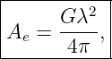
Finally, reciprocity connects transmit gain and receive aperture:
This identity completes the electromagnetic bridge from radiated fields to received power and
prepares the series for Friis transmission, free-space path loss, and RF link budgets.
References
References
[1] Constantine A. Balanis, Antenna Theory: Analysis and Design, 4th ed., Wiley, 2016.
[2] Warren L. Stutzman and Gary A. Thiele, Antenna Theory and Design, 3rd ed., Wiley,
2012.
[3] John D. Kraus and Ronald J. Marhefka, Antennas for All Applications, 3rd ed.,
McGraw-Hill, 2002.
[4] IEEE, IEEE Standard for Definitions of Terms for Antennas, IEEE Std 145-2013,
2014.
[5] David J. Griffiths, Introduction to Electrodynamics, 4th ed., Cambridge University
Press, 2017.




![[U ] = W/sr.](https://images.physicslibrary.org/cache/objects/1451/make4ht/ElectromagneticWavesAntennasAndRFAntennaDirectivityRadiationEfficiencyGainEIRPAndEffectiveAperture4x.png)