Electromagnetic Waves, Antennas, and RF: Polarization of Electromagnetic Waves
EM16 established that a plane electromagnetic wave in vacuum is transverse: the electric field E,
magnetic field B, and propagation direction k are mutually perpendicular. EM17 and EM18 then
showed that the same wave transports energy and momentum. The next question is more
geometric:
That motion defines the polarization of the wave.
For a monochromatic wave traveling in the +z direction, the most general fully polarized
transverse electric field can be written as
where
The amplitudes E0x and E0y and the relative phase δ completely determine the polarization state.
Depending on those three quantities, the tip of E at a fixed point in space traces a line, a circle, or
an ellipse [1, 2, 3, 4].
The central classification is
Linear and circular polarization are therefore special limiting cases of the general polarization
ellipse.
1 Polarization is a transverse-vector property
For propagation in the +z direction, Maxwell’s Equations require
Thus the electric field is confined to the transverse x-y plane. At a fixed spatial location z = z0,
time changes the phase
and therefore changes the two transverse components of E.
Polarization describes the curve traced by the tip of the electric-field vector in that transverse
plane. It is not the path followed by a material particle, and it is not the trajectory of the wave
through space.
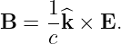
The magnetic field is determined from
so once the electric-field polarization is known, the magnetic-field polarization follows
automatically.
2 Two perpendicular oscillations make one polarization state
Write the two transverse components as
and
The first component establishes one harmonic oscillation along x. The second establishes another
along y. The polarization state is the geometric result of adding these two perpendicular
oscillations.
Three pieces of information matter:
- the x-component amplitude E0x;
- the y-component amplitude E0y;
- the relative phase δ.
The absolute phase ψ determines where the field is in its cycle at a particular instant, but the
polarization shape depends only on relative amplitudes and relative phase.
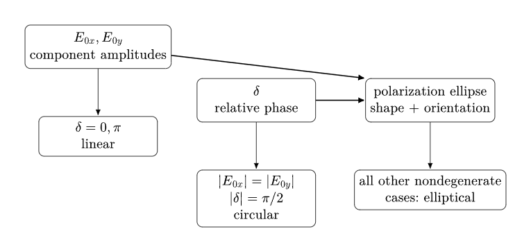
Figure. Two orthogonal amplitudes plus their relative phase determine the polarization
ellipse. Linear and circular polarization are special cases.
3 Linear polarization
Suppose the two components are in phase,
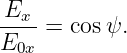
Then
The vector in parentheses is fixed. Only the scalar factor cos ψ changes with time. Therefore the
electric field oscillates back and forth along one fixed line.
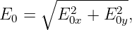
Define
and a polarization angle α such that
Then
The unit polarization vector is
The same linear state also occurs when the components are 180∘ out of phase,
because the two components still remain locked to a fixed line.
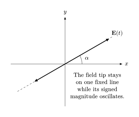
Figure. For linear polarization the electric-field tip remains on a fixed line in the
transverse plane. The field reverses direction every half-cycle.
4 Example 1: a linearly polarized field at 30∘
Let
Then
| E0x | = E0 cos 30∘ = 8.66 V/m, | (18)
|
| E0y | = E0 sin 30∘ = 5.00 V/m. | (19) |
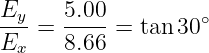
Thus
The ratio
is constant whenever the common cosine factor is nonzero. That constant ratio is the mathematical
signature of a fixed polarization line.
5 Relative phase bends the line into an ellipse
For general phase difference δ, begin with
Expand the y component:
 | = cos(ψ + δ) | (23)
|
| = cos ψ cos δ − sin ψ sin δ. | (24) |
Rearrange:
Square both sides:
Since
we obtain
Expanding and collecting terms gives the polarization-ellipse equation
This single equation contains linear, circular, and general elliptical polarization as special
cases.
6 Circular polarization
Circular polarization requires equal orthogonal component amplitudes,
and a quarter-cycle phase offset,
For
the field components are
and
Therefore
so
The vector magnitude stays fixed while its direction rotates. The tip of E therefore traces a
circle.
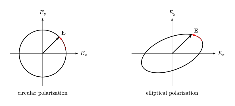
Figure. Equal component amplitudes in quadrature produce a circle. Unequal amplitudes
or a nonquadrature phase offset generally produce an ellipse.
7 Handedness and convention
A rotating electric-field vector has a sense of rotation. Unfortunately, different communities have
historically used different viewing conventions when assigning the labels “right-hand” and
“left-hand.” This article follows the IEEE antenna convention: look in the direction of propagation.
A field that appears to rotate clockwise is called right-hand circularly polarized, while
counterclockwise rotation is called left-hand circularly polarized [5, 3].
Because convention errors are common, a safe technical description should state at least one of the
following explicitly:
- the propagation direction k;
- the actual time-domain component equations;
- the Jones vector and time convention;
- the stated handedness convention.
The words “RHCP” or “LHCP” without a convention can be ambiguous when comparing antenna
and optics literature.
8 Elliptical polarization is the general case
When the components are neither locked to the same line nor arranged as equal-amplitude
quadrature components, the field tip generally traces an ellipse.
The ellipse can be described by
- its major-axis amplitude Emaj;
- its minor-axis amplitude Emin;
- its orientation angle τ;
- its sense of rotation.
The squared semi-axis amplitudes are
The plus sign gives the major axis and the minus sign gives the minor axis.
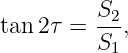
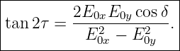
The orientation of the ellipse satisfies
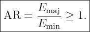
The usual axial ratio is
Thus
is circular polarization, while
approaches linear polarization.
A frequently used logarithmic measure is
9 Example 2: determine an elliptical polarization state
Let
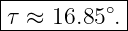
The orientation angle follows from
Hence
so
For the semi-axis amplitudes,
| Emaj2 | =  ![[ ∘ ----------------------]
20 + (12)2 + 4(16)(4)(0.25)](https://images.physicslibrary.org/cache/objects/1442/make4ht/ElectromagneticWavesAntennasAndRFPolarizationOfElectromagneticWaves44x.png) | (47)
|
| = 17.211, | (48)
|
| Emin2 | =  ![[ ∘ ----------------------]
20 − (12 )2 + 4(16)(4)(0.25)](https://images.physicslibrary.org/cache/objects/1442/make4ht/ElectromagneticWavesAntennasAndRFPolarizationOfElectromagneticWaves46x.png) | (49)
|
| = 2.789. | (50) |
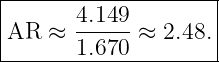
Therefore
and
The axial ratio is
This is clearly elliptical: the axial ratio is finite but greater than unity.
10 Complex notation and the Jones vector
For monochromatic waves it is convenient to encode amplitude and relative phase in complex
numbers. Using the real-field convention
write the complex field amplitude as
The corresponding Jones vector is
If only polarization and not absolute field strength matters, use the normalized Jones
vector
A common overall phase factor does not change the polarization state. Thus
and
represent the same polarization ellipse.
Jones vectors describe deterministic, fully polarized monochromatic fields. Partially polarized or
incoherent fields require a statistical description such as Stokes parameters or a coherency
matrix.
11 Useful Jones-vector special cases
Horizontal linear polarization can be represented as
Vertical linear polarization is
Linear polarization at angle α is
Equal-amplitude quadrature states are
The explicit sign and the adopted ei(kz−ωt) convention determine the rotation sense.
This explicit complex representation is often safer than relying on a handedness label
alone.
12 Stokes parameters as measurable polarization coordinates
For the Jones vector
define the Stokes parameters in the convention used here by
| S0 | = E0x2 + E
0y2, | (65)
|
| S1 | = E0x2 − E
0y2, | (66)
|
| S2 | = 2E0xE0y cos δ, | (67)
|
| S3 | = 2E0xE0y sin δ. | (68) |
For a fully polarized wave,
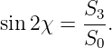
The ellipse orientation and ellipticity angle χ can be written as
and
The limiting values
and
correspond to linear and circular polarization, respectively. The sign of S3 and the associated
handedness label must always be interpreted together with the stated convention.
13 Polarization does not change the basic plane-wave energy relation
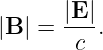
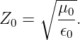
For a vacuum plane wave,
Therefore at every instant
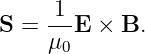
The instantaneous Poynting vector is
For propagation in +z,
where
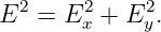
For the general two-component harmonic field,
The cycle averages satisfy
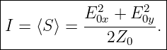
Hence
The relative phase changes the polarization geometry, but for fixed component amplitudes it does
not change the time-averaged intensity.
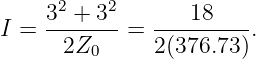
14 Example 3: intensity of a circularly polarized wave
Suppose
with a 90∘ phase difference. Then
Therefore
Notice that the magnitude |E| = 3.0 V/m is constant in time for this circular state. Consequently
the instantaneous power flow is also constant, unlike a single-component linearly polarized sinusoid
whose instantaneous E2 oscillates between zero and its maximum.
15 Polarization and antennas
An antenna is sensitive not only to frequency and direction of arrival but also to polarization. A
receiving antenna couples most strongly when its polarization state matches that of the incident
field.
Let
be the normalized polarization vector of the incoming wave and
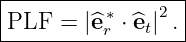
be the normalized polarization state to which the receiving antenna is matched. The polarization
loss factor is
The complex conjugate is required because polarization states can contain relative phase.
The accepted received Power due to polarization alone is reduced by this factor:
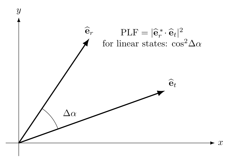
Figure. For two linear polarization directions separated by Δα, the polarization loss factor
becomes cos 2Δα.
16 Linear-polarization mismatch
For linearly polarized transmit and receive states,
and
Their dot product is
| er ⋅et | = cos αr cos αt + sin αr sin αt | (91)
|
| = cos(αt − αr). | (92) |
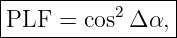
Thus
where
Important special cases are
| Δα = 0∘ | : PLF = 1, | (95)
|
| Δα = 45∘ | : PLF =  , , | (96)
|
| Δα = 90∘ | : PLF = 0. | (97) |
The corresponding mismatch loss in decibels is
17 Example 4: a 30∘ polarization mismatch
Suppose a linearly polarized wave reaches a linear receiving antenna with
Then
Thus the receiver captures 75% of the power that it would capture under perfect polarization
alignment, all else being equal.
The mismatch loss is
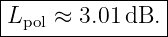
Therefore
18 Circular polarization and linear antennas
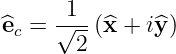
Take a normalized circular state
and a normalized linear state at arbitrary angle α,
Then
| eℓ∗⋅e
c | =   . . | (105) |
Its magnitude squared is
Therefore
which corresponds to
The result is independent of the linear antenna’s orientation angle. A circularly polarized wave
always contains equal power in any pair of orthogonal linear basis directions.
19 Matched and opposite circular polarization
For two identical normalized circular Jones vectors,
so
For the opposite circular state, the two normalized Jones vectors are orthogonal in the complex
inner-product sense. Therefore
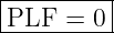
for ideal opposite-handed circular polarizations.
Real antennas are never perfect. Their finite axial ratio, multipath, reflections, radome effects,
platform blockage, and propagation medium can all convert one polarization state into another, so
practical rejection is finite rather than infinite.
20 How circular polarization can be produced
The component picture immediately suggests a physical method. Use two orthogonal
radiating elements that produce equal field amplitudes and drive them with a 90∘ phase
difference.
Symbolically,
The same principle appears in crossed dipoles, turnstile antennas, quadrature-fed patches, and
many other antenna structures. The antenna geometry creates two orthogonal transverse field
components; the feed network or structural mode relationship establishes the relative
phase.
This is an important bridge from plane-wave physics to antenna engineering: polarization is not
an additional property pasted onto Maxwell’s equations. It emerges directly from the
relative amplitude and phase of transverse field components generated by the antenna
currents.
21 Propagation direction and polarization must be stated together
Handedness reversals can appear when the propagation direction is reversed or when the field is
viewed from the opposite side. Therefore a polarization statement is incomplete unless the
propagation direction is known.
For a plane wave,
If k changes sign while the coordinate axes are held fixed, the relationship between phase
progression and observed field rotation must be reconsidered. This is one reason polarization
bookkeeping becomes important in reflected waves, radar, multipath channels, and satellite
links.
22 Common mistakes
- Treating polarization as the path of the wave. Polarization is the motion of the
transverse field vector at a point.
- Ignoring relative phase. Two perpendicular components with the same amplitudes
can produce linear, circular, or elliptical polarization depending on δ.
- Calling every equal-amplitude state circular. Equal amplitudes are not enough;
the phase difference must also be ±90∘.
- Forgetting that linear polarization is a limiting ellipse. The minor axis tends
to zero and the axial ratio tends to infinity.
- Forgetting the viewing convention for handedness. Always specify propagation
direction and convention.
- Using an ordinary dot product for complex polarization vectors. The receiving
polarization overlap uses the complex-conjugate inner product.
- Confusing amplitude loss with power loss. Polarization loss factor is a power
ratio, so decibel loss uses 10 log 10.
- Assuming polarization changes vacuum wave speed. In isotropic vacuum all
polarization states propagate at the same speed c.
23 A compact polarization hierarchy
The main ideas can be summarized as
| two transverse components | →relative amplitude and phase | (114)
|
| →polarization ellipse | (115)
|
| →linear, circular, or elliptical state | (116)
|
| →Jones/Stokes representation | (117)
|
| →antenna polarization matching. | (118) |
The electromagnetic-wave sequence has now progressed from field generation and Maxwell’s
equations to wave propagation, energy, momentum, and finally the internal transverse geometry of
the wave itself.
24 What EM19 adds to the series
EM19 adds the following pieces to the electromagnetic-wave framework:
- polarization defined as transverse electric-field-vector motion;
- linear, circular, and elliptical polarization derived from two orthogonal harmonic
components;
- the polarization ellipse derived algebraically;
- ellipse orientation and axial ratio;
- an explicit handedness convention and warning about convention differences;
- Jones vectors for fully polarized monochromatic fields;
- a first Stokes-parameter representation;
- the fact that average intensity depends on component amplitudes but not relative
phase;
- polarization loss factor and its antenna interpretation;
- the cos 2Δα law for linear mismatch;
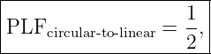
- the 3 dB circular-to-linear mismatch result;
- the connection between quadrature-fed orthogonal antenna modes and circular
polarization.
A natural next step is to study how polarization changes at interfaces and in matter: reflection,
transmission, birefringence, wave plates, and polarization-dependent propagation. In the RF
branch, the same machinery leads directly to antenna polarization purity, axial ratio, multipath
polarization change, and link-budget mismatch losses.
References
References
[1] D. J. Griffiths, Introduction to Electrodynamics, 4th ed., Cambridge University Press,
2017.
[2] J. D. Jackson, Classical Electrodynamics, 3rd ed., Wiley, 1999.
[3] C. A. Balanis, Antenna Theory: Analysis and Design, 4th ed., Wiley, 2016.
[4] W. L. Stutzman and G. A. Thiele, Antenna Theory and Design, 3rd ed., Wiley, 2012.
[5] IEEE, IEEE Standard for Definitions of Terms for Antennas, IEEE Std 145-2013,
2014.




















![( )2 [ ( )2 ]
Ey--− -Ex- cosδ = 1 − Ex-- sin2 δ.
E0y E0x E0x](https://images.physicslibrary.org/cache/objects/1442/make4ht/ElectromagneticWavesAntennasAndRFPolarizationOfElectromagneticWaves24x.png)








![|-----------1-[------------∘------------------------------]--|
|E2maj,min = -- E20x + E20y ± (E20x − E20y)2 + 4E20xE20y cos2δ .
------------2------------------------------------------------|](https://images.physicslibrary.org/cache/objects/1442/make4ht/ElectromagneticWavesAntennasAndRFPolarizationOfElectromagneticWaves33x.png)










![|----[------]--|
| E0x |
|J = E eiδ .|
--------0y-----](https://images.physicslibrary.org/cache/objects/1442/make4ht/ElectromagneticWavesAntennasAndRFPolarizationOfElectromagneticWaves52x.png)
![|-----------------[------]-|
| 1 E0x |
^J = ∘----------- E eiδ .|
| E20x + E20y 0y |
----------------------------](https://images.physicslibrary.org/cache/objects/1442/make4ht/ElectromagneticWavesAntennasAndRFPolarizationOfElectromagneticWaves53x.png)


![|----------|
| [1] |
|^Jx = .|
-------0----](https://images.physicslibrary.org/cache/objects/1442/make4ht/ElectromagneticWavesAntennasAndRFPolarizationOfElectromagneticWaves56x.png)
![|----------|
| [0] |
|^Jy = .|
-------1----](https://images.physicslibrary.org/cache/objects/1442/make4ht/ElectromagneticWavesAntennasAndRFPolarizationOfElectromagneticWaves57x.png)
![|------[-----]-|
| cosα |
^Jlin = sin α .|
----------------](https://images.physicslibrary.org/cache/objects/1442/make4ht/ElectromagneticWavesAntennasAndRFPolarizationOfElectromagneticWaves58x.png)
![|---------[---]--|
|^ -1-- 1 |
|J± = √ -- ±i .|
---------2-------](https://images.physicslibrary.org/cache/objects/1442/make4ht/ElectromagneticWavesAntennasAndRFPolarizationOfElectromagneticWaves59x.png)
![[ ]
J = E0x ,
E0yeiδ](https://images.physicslibrary.org/cache/objects/1442/make4ht/ElectromagneticWavesAntennasAndRFPolarizationOfElectromagneticWaves60x.png)