Degrees of Freedom in Mechanics
A mechanical system may be described with many coordinates, but not all of those
coordinates are necessarily independent. The number of degrees of freedom is the
minimum number of independent parameters required to specify the configuration of the
system.
This idea becomes increasingly important as mechanics progresses. It explains why a pendulum
needs only one generalized coordinate, why a free particle in three-dimensional space needs three,
why a rigid body in space needs six, and why constraints can reduce a seemingly complicated
problem to a much smaller one.
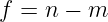
The basic counting idea is
For a system initially described by n coordinates and subject to m independent regular holonomic
constraints, the local count is
This formula is powerful, but its assumptions matter. The constraints must actually be
independent, and more advanced nonholonomic or singular constraints require greater
care.
1 Coordinates are not automatically degrees of freedom
Suppose a particle moves in the xy plane. Its position can be specified by two Cartesian
coordinates,
so an unconstrained particle in a plane has two degrees of freedom.
Now suppose the particle is restricted to a circle of fixed radius L:
Although two Cartesian coordinates still appear, they are not independent. Once x is chosen, y is
restricted by the constraint, and vice versa. A single angular coordinate 𝜃 can describe the
configuration:
The constrained particle therefore has one degree of freedom.
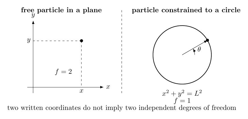
Figure 1. Coordinates and degrees of freedom are not the same thing. A free particle in a plane
needs two independent coordinates, while a particle constrained to a circle needs only one.
2 Configuration versus state
The word configuration refers to where the system is geometrically, not to how fast it is
moving.
For a particle moving along a line, one coordinate x specifies its configuration. The system
therefore has one configuration degree of freedom.
To predict future motion using Newtonian mechanics, one normally also needs the velocity ẋ.
Thus the instantaneous dynamical state can be represented by
That does not mean the particle suddenly has two configuration degrees of freedom. It still has one
degree of freedom; position and velocity together specify its state.
In hamiltonian mechanics a system with f configuration degrees of freedom is commonly
represented in a 2f-dimensional phase space with coordinates
This distinction between configuration-space dimension f and phase-space dimension 2f is
important later in analytical mechanics.
3 Elementary examples
Several common systems provide useful reference points.
A particle restricted to a straight line has
A free particle in a plane has
A free particle in ordinary three-dimensional space has
Two independent free particles in three dimensions require six independent position coordinates,
so
For N unconstrained particles in three dimensions,
Constraints reduce this number.
4 Constraints reduce the number of independent coordinates
A constraint restricts the configurations available to a system. A holonomic constraint can be
written as an equation involving the coordinates and possibly time:
If there are m independent holonomic constraints,
then, under regular conditions, the number of independent degrees of freedom is
The word independent matters. Repeating the same physical constraint in different algebraic forms
does not remove extra degrees of freedom.
5 Worked example 1: the simple pendulum
A point mass moving in a vertical plane has Cartesian coordinates (x,y), so without constraints it
would require two degrees of freedom.
For a pendulum of fixed length L, the mass must satisfy
There are two coordinates and one independent holonomic constraint, so
A convenient generalized coordinate is the angle 𝜃:
Once 𝜃 is specified, both Cartesian coordinates are fixed. The pendulum therefore has one degree
of freedom.
This example captures the main advantage of generalized coordinates: instead of carrying two
coordinates plus a constraint equation, one may choose a single coordinate that automatically
satisfies the constraint.
6 Configuration space
For a system with f degrees of freedom, the set of all allowed configurations forms an
f-dimensional configuration space.
For a free particle in a plane, configuration space is the entire xy plane. For a particle
constrained to a circle, the allowed configurations form only the circle itself, which is
one-dimensional.
The system may be embedded in a higher-dimensional coordinate space while its actual
configuration space has lower dimension because of constraints.
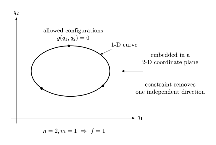
Figure 2. A constraint can reduce the dimension of configuration space. The circle is embedded in
a two-dimensional plane but is itself a one-dimensional configuration space.
7 Generalized coordinates
A set of independent variables
that uniquely specifies the configuration is called a set of generalized coordinates.
Generalized coordinates do not have to be Cartesian distances. They may be angles, lengths along
a curve, rotation parameters, or combinations of ordinary coordinates.
For example, a bead constrained to move on a fixed wire can often be described by a single path
coordinate s. A pendulum can be described by one angle 𝜃. A planar rigid body can be described
by two translation coordinates and one orientation angle.
The number of generalized coordinates required equals the number of degrees of freedom, provided
the coordinates are independent and nonsingular in the region of interest.
8 Worked example 2: three particles forming a rigid triangle in a plane
Consider three point masses moving in a plane. Without constraints, each mass needs two
coordinates, so the three-particle system has
coordinates.
Now suppose the three pairwise distances are fixed:
For a nondegenerate triangle these are three independent geometric constraints. Therefore
Those three degrees of freedom have a simple physical interpretation:
- translation of the whole triangle in the x direction,
- translation of the whole triangle in the y direction,
- rotation of the triangle in the plane.
Thus a rigid body moving in a plane has three degrees of freedom.
9 Rigid bodies
A rigid body contains an enormous number of atoms, but its internal distances are fixed to an
excellent approximation. Those rigidity constraints remove almost all of the particle
coordinates.
A rigid body moving freely in three-dimensional space has six degrees of freedom:
Three specify translation of a reference point, such as the center of mass:
Three specify orientation.
Orientation may be represented in many ways: Euler Angles, a direction-cosine matrix, an
axis-angle description, or a quaternion. Some of those representations use more numerical
parameters than three, but extra algebraic constraints may be present. The physical orientation
still has three degrees of freedom.
A unit quaternion, for example, uses four numbers but obeys one normalization condition.
Therefore its four components do not represent four independent rotational degrees of
freedom.
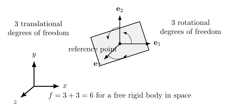
Figure 3. A free rigid body in three-dimensional space has six degrees of freedom: three
translational and three rotational.
10 Worked example 3: a rigid dumbbell in three dimensions
Two point masses in three-dimensional space have six unconstrained coordinates:
Suppose they are connected by a massless rigid rod of fixed length L. The distance constraint
is
This is one independent constraint, so
The result also has a direct physical interpretation. Three coordinates locate the center of mass.
Two angles specify the direction of the rod in space. Rotation about the rod’s own axis
does not change the configuration of two point masses, so no sixth degree of freedom
appears.
This contrasts with a general three-dimensional rigid body, whose material distribution can change
orientation under rotation about any of its body axes and therefore requires three independent
orientation degrees of freedom.
11 Degrees of freedom and symmetries
A degree of freedom describes an independent way the configuration can change. A symmetry can
make the associated coordinate dynamically simple, but symmetry does not automatically remove
the degree of freedom.
For example, the azimuthal angle of a particle in a central force field remains a valid
coordinate even if the Lagrangian does not depend explicitly on that angle. The coordinate
is then cyclic, and its conjugate momentum is conserved. The degree of freedom still
exists.
Thus it is useful to distinguish
from
12 When the simple counting rule needs care
The formula
Works well for independent regular holonomic constraints. Several situations require more careful
analysis.
Redundant constraints
If one constraint follows from the others, it does not reduce the dimension again.
Singular configurations
At special geometric configurations, the rank of the constraint equations may change. A counting
formula valid in a regular region can then fail at the singular point.
Nonholonomic constraints
Some constraints involve velocities and cannot be integrated into coordinate-only equations.
Rolling without slipping is a standard example. Advanced mechanics distinguishes carefully
between the dimension of configuration space and the instantaneous velocity directions permitted
by such constraints.
For the introductory use of degrees of freedom, the safest rule is to count independent coordinates
after incorporating all independent geometric constraints.
13 Degrees of freedom in continua and fields
A continuous string, fluid, or electromagnetic field is described by a quantity defined at every
spatial point. Such systems are often said to possess infinitely many degrees of freedom in the
continuum idealization.
A vibrating string, for example, is described by a displacement field
Discretizing the string into N movable masses produces approximately N coordinates. Taking the
continuum limit sends the number of coordinates toward infinity.
This is one bridge from particle mechanics to continuum mechanics and classical field
theory.
14 Degrees of freedom and normal modes
Near stable equilibrium, a system with f mechanical degrees of freedom often has f independent
small-oscillation normal modes, after appropriate treatment of constraints and zero-frequency
symmetries.
This connection will become important in the later small-oscillation sequence. Degrees of freedom
determine the dimension of the coordinate problem; normal modes provide a particularly useful set
of coordinates for the linearized dynamics.
15 A practical counting procedure
For elementary mechanics problems, the following procedure is reliable.
- Identify the objects whose configurations must be specified.
- Count the coordinates before constraints are applied.
- Write the independent geometric constraints explicitly.
- Subtract only independent constraints.
- Check whether a smaller set of generalized coordinates can describe the allowed
configurations directly.
- Verify that changing any one proposed generalized coordinate can change the
configuration independently, at least locally.
The process can be summarized as
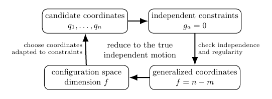
Figure 4. Degrees-of-freedom counting is a reduction from a possibly redundant coordinate
description to the independent coordinates that span the allowed configuration space.
16 Common mistakes
- Counting every written coordinate as an independent degree of freedom.
- Counting velocities as extra configuration degrees of freedom.
- Subtracting constraints that are algebraically redundant.
- Assuming a four-component quaternion means four rotational degrees of freedom.
- Confusing a conserved coordinate momentum with removal of the coordinate itself.
- Applying f = n−m blindly to singular or nonholonomic systems without checking its
assumptions.
17 Practice problems
M00-07-P01: Particle on a line
A particle is constrained to move along the x axis. How many configuration degrees of freedom
does it have? Give one possible generalized coordinate.
M00-07-P02: Particle on a sphere
A particle moves on the surface of a sphere of fixed radius R. Starting from Cartesian
coordinates (x,y,z), count the degrees of freedom and suggest a convenient pair of generalized
coordinates.
M00-07-P03: Two free particles in a plane
Two independent particles move in a plane. How many degrees of freedom does the system
have?
M00-07-P04: Two particles joined by a rigid rod in a plane
Two point masses move in a plane and remain separated by a fixed distance L. Count the degrees
of freedom. Interpret them physically.
M00-07-P05: Bead on a rotating hoop
A bead is constrained to a circular hoop of fixed radius. The hoop’s rotation angle is prescribed
externally as a known function of time. How many mechanical configuration degrees of freedom
does the bead have?
M00-07-P06: Planar rigid body
Explain why a general rigid body moving in a plane has three degrees of freedom. Name a
convenient set of generalized coordinates.
M00-07-P07: Spatial rigid body
A free rigid spacecraft is modeled as a rigid body in three-dimensional space. How many degrees of
freedom does its configuration have? Explain why a four-component unit quaternion does not
change that physical count.
M00-07-P08: Constrained particle system
Four particles move in three dimensions. Before constraints are applied, how many degrees of
freedom are available? If three independent holonomic constraints are imposed, what is the local
degree-of-freedom count?
18 Short answer check
- P01: one; for example x.
- P02: two; for example spherical angles 𝜃 and ϕ.
- P03: four.
- P04: three; two translations plus one orientation angle.
- P05: one, because the hoop motion is prescribed rather than an independent dynamical
coordinate.
- P06: three; for example (xCM,yCM,𝜃).
- P07: six; the quaternion has four components plus one normalization constraint, leaving
three independent orientation parameters.
- P08: twelve before constraints and nine after three independent constraints.
19 Where this article leads
Degrees of freedom are the natural bridge from elementary Newtonian mechanics to analytical
mechanics. The next conceptual steps are generalized coordinates, constraints, virtual
displacements, and Lagrange’s equations. Later articles will also use the same counting ideas for
rigid-body dynamics, small oscillations, Hamiltonian phase space, continuum mechanics, and field
theory.
References
[1] J. R. Taylor, Classical Mechanics, University Science Books, 2005.
[2] J. B. Marion and S. T. Thornton, Classical Dynamics of Particles and Systems, 5th
ed., Brooks/Cole, 2004.
[3] H. Goldstein, C. Poole, and J. Safko, Classical Mechanics, 3rd ed., Addison-Wesley,
2002.
[4] Wikibooks, Classical Mechanics, sections on generalized coordinates and constraints,
CC BY-SA.