E03: Electrical Resistance and Ohm’s Law
Foundations of Electricity and Electrical Measurement, mini-lecture 3.
E01 introduced voltage as a potential difference, and E02 identified electric current with the rate of
transported charge. When a voltage is placed across a piece of conducting material, what
determines the resulting current?
A Conductor does not respond only to the applied voltage. Its material, shape, and temperature
also matter. Those effects are described by resistivity and resistance. For a broad class of materials
under well-controlled conditions, the current is proportional to the voltage. This is Ohm’s
law.
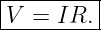
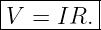
The circuit-level equation is
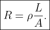
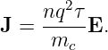
The corresponding local material relationship is
The goal of this lecture is not just to use the first equation. We will derive its connection to the
second, examine where both relationships apply, and explain how to measure resistance in a real
laboratory.
Learning objectives
- distinguish resistance of a component from resistivity of a material;
- explain why a current-carrying conductor can have a nonzero internal Electric Field;
- derive R = ρL∕A and V = IR from local conduction;
- connect a simple drift model to conductivity;
- interpret the slope of a current-versus-voltage graph;
- account for temperature and distinguish ohmic from non-ohmic devices;
- calculate resistor heating and verify a Power rating;
- distinguish two-wire and four-wire measurements, and avoid meter-loading errors in
EDL01.
1 From the electric field to moving charge
Consider a uniform metal rod connected between two terminals. If the left terminal is at higher
electric potential, the electric field inside the rod points approximately from left to right. Electrons
have charge −e and drift slowly to the left. Their motion produces conventional current toward the
right, as discussed in E02.
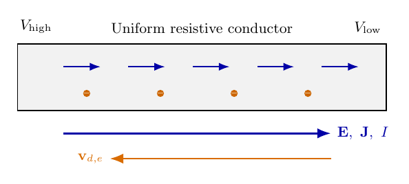
Figure 1. A maintained voltage drop creates an internal electric field. Electron drift is opposite to
conventional current and to the field in an ordinary metal.
The average electron drift is small compared with the electrons’ random microscopic motion. In a
metal, interactions with the lattice, impurities, and other scattering processes limit the directed
drift. The resulting current can remain steady even though an electric field exerts a force on each
carrier.
There is an important distinction from the electrostatics of E01. In an ideal conductor in
electrostatic equilibrium, E = 0 inside the bulk. A resistive conductor carrying a steady current is
not in electrostatic equilibrium: it generally has E≠0 within the material.
2 Current density and the local form of Ohm’s law
Current density J measures conventional current per unit area and points along the direction of
positive charge transport. In a uniform wire of cross-sectional area A, with uniform current density
parallel to its axis,
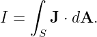
The full relation from E02 is
For many isotropic conductors at fixed temperature, over a useful range of fields, experiments find
that current density is proportional to the field:
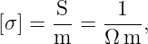
Here σ is the electrical conductivity. Its SI unit is
where S denotes the siemens.
The reciprocal is the electrical resistivity ρ:
Consequently,
Resistivity has SI unit Ω m. A material with low resistivity can carry more current at the
same electric field than a material with high resistivity. For a homogeneous isotropic
material, ρ is a scalar; more complex materials may require conductivity and resistivity
tensors.
3 Deriving resistance from material and geometry
Take a straight, uniform conducting specimen of length L and cross-sectional area A. Assume that
ρ is constant within the specimen, the current density is approximately uniform, and the DC
conduction field is axial. From the potential-field relation of E01,
With a uniform field directed along the specimen,
Similarly, the current is
Substitute E = ρJ:
| V | = EL, | (12)
|
| = ρJL, | (13)
|
| = ρ L, | (14)
|
| =  I. | (15) |
The quantity multiplying the current is the specimen’s electrical resistance:
Therefore,
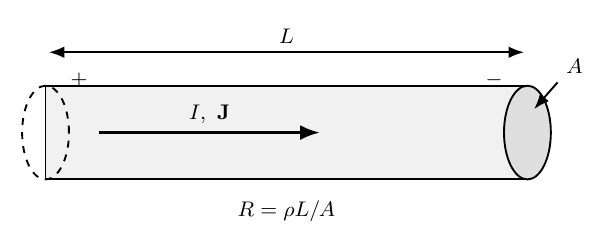
Figure 2. Resistance depends on specimen length L, area A, and resistivity ρ. At fixed material
and temperature, increasing L raises resistance while increasing A lowers it.
The resistance is a property of the particular object, including its geometry. Resistivity is
a property of the material under specified conditions. The formula R = ρL∕A is not
universal for arbitrary shapes, nonuniform fields, contact resistances, or strongly nonlinear
conductors.
3.1 Units and a numerical example
Since R = V∕I, its unit is the ohm:
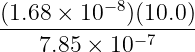
At approximately 20 ∘C, a representative resistivity for copper is 1.68 × 10⁻⁸ Ω m. A 10.0 m
length of copper wire with diameter 1.00 mm has area
Its approximate resistance is
| R | = ρ , | (20)
|
| =  Ω, | (21)
|
| ≈ 0.214 Ω . | (22) |
The result is a resistance for the specified length, not a universal “resistance of copper.”
4 Why conductivity arises: a simple drift model
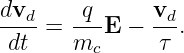
A basic microscopic model helps explain the observed proportionality. Let a carrier have mass mc,
signed charge q, and an average momentum relaxation time τ. In the simplest collision model, the
mean drift velocity obeys
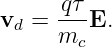
In steady state, dvd∕dt = 0, so
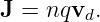
With carrier number density n, E02 gives
Combining the expressions,
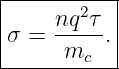
Thus this simplified model predicts
For electrons, q = −e, but q2 is positive. An electron drifts opposite to the field while the
conventional current density points along the field.
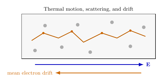
Figure 3. Random carrier motion is accompanied by a small average drift. Scattering limits
directed motion, giving a finite conductivity in the simple relaxation-time model.
This is a useful model, not a complete theory of metallic conduction. Real materials require
additional microscopic physics to predict the actual value and temperature dependence of
σ.
5 What Ohm’s law says, and what it does not say
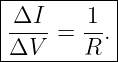
If R is constant over an experimental range, then I = V∕R. A graph of current I on the vertical
axis against voltage V on the horizontal axis is a straight line through the origin with
slope
By contrast, if voltage is plotted vertically against current, the slope is R. One must read the axis
labels before interpreting a measured slope.
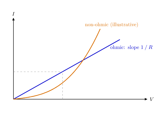
Figure 4. On an I-versus-V plot, the straight line represents an ohmic element with constant R. A
curved characteristic indicates a voltage- or current-dependent response.
Ohmic behavior means an approximately linear current-voltage relationship at fixed physical
conditions. It is an empirical material or device behavior, not a universal consequence of
conservation of charge. A diode, heated lamp filament, and many semiconductor devices are
non-ohmic under ordinary operating conditions.
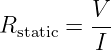
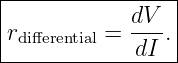
For nonlinear devices, two different quantities are often useful:
and
The first measures the ratio at one operating point (when I≠0), while the second describes the
local incremental response. These need not be equal. For a linear ohmic resistor, both reduce to the
same constant R.
6 How temperature changes resistance
Resistivity depends on temperature. Over a sufficiently narrow range, the resistivity of many
metals is approximately
where ρ0 is the resistivity at reference temperature T0 and α is a temperature coefficient in K−1. If
changes in specimen dimensions are negligible, the same approximation gives
For copper near room temperature, a representative value is α ≈ 3.9 × 10⁻³ K−1. With a 100 Ω
reference resistance at 20 ∘C, the model predicts at 60 ∘C:
| R | ≈ (100)[1 + (0.0039)(60 − 20)] Ω, | (33)
|
| ≈ 115.6 Ω . | (34) |
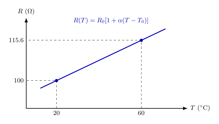
Figure 5. The local linear approximation for copper-like resistance increases with temperature. It
is not intended as a universal formula over arbitrary temperature ranges.
For a metal, greater thermal scattering commonly reduces carrier mobility. Some semiconductors
and thermistors instead exhibit decreasing resistance with increasing temperature. In general, a
resistor also warms due to its own electrical power dissipation, so an apparently nonlinear
I-versus-V curve may result from changing temperature during a measurement.
7 Conductance and power dissipation
The reciprocal of resistance is called conductance:
Its SI unit is the siemens, S = Ω−1. Conductance is a property of a component. Conductivity, σ, is
a material property with units S∕m.
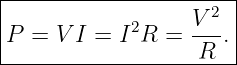
Electric power delivered to a two-terminal component is P = V I when the current
enters the terminal labeled at higher voltage (passive sign convention). For an ohmic
resistor,
This electrical energy is predominantly transferred into thermal energy. E04 develops the power
and energy bookkeeping in detail.
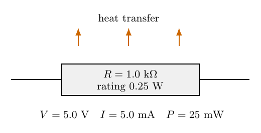
Figure 6. A resistor has a nominal resistance, tolerance, and finite power rating. At fixed voltage
its idealized dissipated power is V 2∕R; the rating must not be exceeded.
For example, applying 5.0 V across a 1.0 kΩ resistor produces
| I | =  = 5.0 mA, | (37)
|
| P | =  = 0.025 W. | (38) |
This is below a 0.25 W nominal resistor rating, although appropriate margins and environmental
derating still matter.
8 Measuring resistance in the laboratory
8.1 Voltage-current measurement
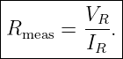
A direct experimental estimate of resistance is
A voltmeter measures voltage in parallel with the component; an ammeter measures current in
series. A digital multimeter (DMM) typically has a large finite input resistance in voltage mode,
and a finite internal burden in current mode. Therefore both instruments can perturb the circuit,
particularly at very large or very small resistances.
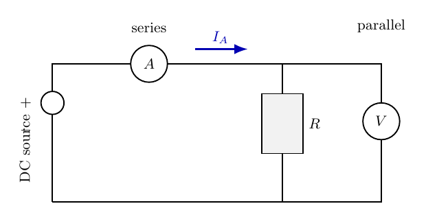
Figure 7. An ammeter is inserted in series; a voltmeter connects across the selected resistor. Never
place an ammeter directly across a voltage source.
With the indicated arrangement, the ammeter reads the resistor current plus the small current
drawn by the voltmeter. Thus V∕Imeter slightly underestimates the resistor’s actual resistance. For
typical DMM inputs and kilohm resistors, the effect may be small; for high resistances, it can
matter.
8.2 Ohmmeter mode and unwanted parallel paths
A DMM in ohmmeter mode applies an internal test stimulus and senses the response.
Disconnect the power source and discharge capacitors before using resistance mode. Whenever
possible, isolate one end of the component because other circuit paths may appear in
parallel.
For example, if the intended 1.0 kΩ resistor remains in parallel with another 1.0 kΩ resistor, the
in-circuit reading is approximately
A 500 Ω reading would not imply that either component is defective.
8.3 Two-wire and four-wire measurements
At small resistances, the leads and contacts add a measurable contribution:
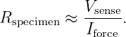
In a four-wire or Kelvin measurement, one pair of conductors carries the test current and
a separate high-input-resistance pair senses voltage across the specimen. In the ideal
limit,
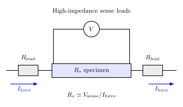
Figure 8. Four-wire resistance measurement keeps the voltage-sensing leads separate from the
current-carrying leads, reducing the influence of lead voltage drops.
High input impedance minimizes current in the voltage-sensing leads. Real four-terminal setups
still require attention to contact placement, offset voltages, heating, and instrument
specifications.
9 EDL01 bridge: a low-voltage Ohm’s-law experiment
A suitable first experiment uses a 1.0 kΩ, 0.25 W resistor, a current-limited adjustable DC supply
(or suitable batteries), and a DMM. Use a low-voltage range such as 0 to 5 V. Verify
resistor value with power disconnected, then wire the powered circuit. Do not use mains
voltage.
- Record the resistor’s nominal value, tolerance, and the DMM range.
- Set the source to 0 V and connect the resistor and meter following the proper series
or parallel measurement configuration.
- Measure the resistor voltage and the associated current at successive settings from 0
to 5 V.
- Plot I versus measured V R. Fit the nonzero-current data to I = aV R + b, checking
whether b is consistent with zero.
- Estimate resistance from R ≈ 1∕a when b is negligible and instrument loading is small.
- Compare the result with the ohmmeter reading and resistor tolerance.
A reasonable ideal expectation is
At 5.0 V, this gives 5.0 mA and 25 mW. Do not assume that the supply-panel display equals the
measured voltage across the resistor. Wires, source impedance, and meter burden may produce
additional voltage drops.
10 Common misconceptions
- A resistor does not consume current. Charge continuity still holds; electrical energy is
transferred to other forms.
- R and ρ are not interchangeable. Resistance includes object geometry; resistivity
describes material response.
- The equation V = IR is not a universal law for every device at all currents, voltages,
and temperatures.
- The slope of an I-versus-V graph is 1∕R, not R.
- A steady current in an ordinary metal generally requires a nonzero internal electric
field.
- A DMM changes the circuit to some extent; its voltage, current, and resistance modes
are not interchangeable.
- Measuring resistance on a powered circuit is unsafe and can damage the meter.
11 Summary and next steps
The core connections are
For simple drift kinetics, σ = nq2τ∕m
c explains why density and mobility matter. Temperature,
nonuniform geometry, nonlinear materials, and instrument loading determine how accurately the
simplified relations represent a particular experiment.
E03E1 provides worked problems and solutions. E04 will examine electrical power and energy in
greater detail; E05-E08 will expand to connected circuits and nonideal sources. EDL01 supplies the
related measurements.
References
References
[1] OpenStax, University Physics, Volume 2, §9.3, “Resistivity and Resistance,” (online
textbook).
[2] OpenStax, University Physics, Volume 2, §9.4, “Ohm’s Law,” (online textbook).
[3] D. J. Griffiths, Introduction to Electrodynamics, chapters on currents and fields in
matter.