Sampling, Aliasing, and the Nyquist-Shannon Sampling Theorem
A continuous signal contains information at every instant of time. A digital instrument stores only
a sequence of numbers. How can those numbers preserve an entire continuous waveform? The
Nyquist-Shannon sampling theorem gives a surprisingly precise answer, provided we state the
assumptions carefully.
The key result is not that any curve can be reconstructed from two points per cycle. Rather, a
signal whose Fourier transform vanishes outside a known frequency band can, under ideal sampling
conditions, be determined from equally spaced samples taken sufficiently fast. The theorem is a
statement about the structure of the signal’s entire spectrum.
We will build the result in the same manner as the preceding PhysicsLibrary Fourier series
lectures:
- begin with a single sinusoid and discover frequency ambiguity;
- interpret sampling as multiplication by a periodic impulse train;
- derive why sampling creates shifted copies of the Fourier spectrum;
- obtain the sampling-rate condition by demanding that the copies not overlap;
- recover the signal using an ideal low-pass filter and sinc interpolation;
- apply the results to a force pulse and to a practical electronics-lab experiment.
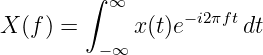
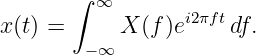
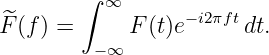
We will use the Fourier-transform convention
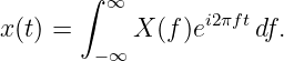
and the corresponding inverse
The frequency variable f is in cycles per second, or hertz. Using angular frequency ω = 2πf gives
an equivalent convention with different factors of 2π.
1 Definitions and the sampling question
A sampling period Ts is the uniform time interval between successive measurements. The sampling
frequency is
The samples of a continuous-time signal x(t) are
square brackets signal a discrete-time sequence; parentheses signal the continuous-time function.
The integer n counts samples, while t measures physical time.
A signal is band-limited to B hertz when its Fourier transform satisfies
For the easiest reconstruction statement we assume the signal is supported strictly inside the
sampled baseband, so that a nonzero guard region separates its spectrum from the copies created
by sampling.
The Nyquist frequency is half the sample rate:
The nominal Nyquist rate of a signal band-limited to B is 2B samples per second. A robust strict
nonoverlap condition is fs > 2B. The equality case needs separate attention because
content exactly at the band edge can be ambiguous for some signal classes and sample
phases.
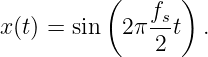
2 Two continuous signals can have identical samples
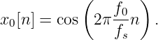
Consider the real sinusoid
Sampling at t = nTs = n∕fs gives
Now choose another continuous frequency
where k is any integer. Its samples are
| x1[n] | = cos 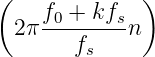 | (10)
|
| = cos 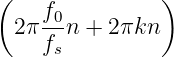 | (11)
|
| = cos  . | (12) |
The last line follows because kn is an integer and adding an integral multiple of 2π does not change
a cosine.
This is aliasing: distinct continuous-frequency components can become indistinguishable after
uniform sampling. The ambiguity is not caused by imperfect arithmetic or a noisy instrument. It is
present even in exact mathematical samples.
Worked example: 100 Hz versus 900 Hz
Let fs = 1000 Hz, so Ts = 1 ms. Sample two signals:
The samples are
and
| xb[n] | = cos(1.8πn) | (16)
|
| = cos(2πn − 0.2πn) | (17)
|
| = cos(0.2πn). | (18) |
Thus every sample is identical, although the continuously varying functions are quite different
between sample times.
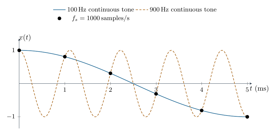
Figure 1. Two different continuous cosine signals have the same values at the marked sampling
instants. The sample sequence cannot distinguish a 100 Hz tone from a 900 Hz cosine when
sampled at 1000 samples per second.
The same conclusion follows from the identity
For sines, the reflected-frequency contribution may have a sign reversal rather than the
same samples. The positive/negative-frequency viewpoint will make this distinction
systematic.
3 Why one half of the sample rate is special
For a complex exponential,
Uniform sampling therefore identifies frequencies differing by integer multiples of fs. We can select
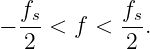
a representative interval of width fs:
For a real signal, positive and negative complex-frequency contributions are paired. A real sampled
cosine at fs − f0 has the same samples as one at f0.
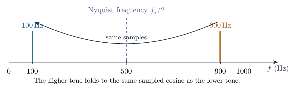
Figure 2. The 900 Hz tone folds into the 100 Hz sampled-cosine pattern at fs = 1000 Hz. The
marked Nyquist frequency is 500 Hz.
The alias frequency of a positive real sinusoid can be found by shifting its frequency by a suitable
integer multiple of fs and folding the result into [0,fs∕2]. One convenient rule is to choose an
integer k for which
lies in the Nyquist band. For the example above, k = 1 gives
This rule describes the observed frequency of an aliased sinusoidal component. It is not a means of
recovering the true input frequency from the samples alone.
4 Why a single-sinusoid argument is not enough
Real signals are normally mixtures of frequencies. A vibration record, received radio signal, or
output of a function generator may contain many sinusoidal components at once. We
need to understand what sampling does to the entire spectrum X(f), not only to one
tone.
The inverse Fourier transform from Equation (2) writes the signal as a continuous superposition:
This is the same philosophical step developed in the Fourier series-to-transform lecture FS26. A
periodic signal has discrete spectral frequencies; a general nonperiodic signal can require a
continuum of frequencies. Sampling imposes a new periodic structure on that continuous
spectrum.
5 Represent ideal sampling with an impulse train
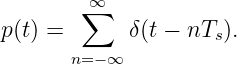
An ideal mathematical sampler can be modeled by the sampling impulse train, also called a Dirac
comb:
Here δ is the Dirac delta distribution. The sifting identity is
The impulse train is not an ordinary finite-amplitude electrical waveform. It is an idealization that
retains sample values while simplifying Fourier analysis.
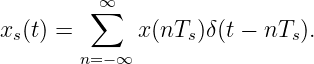
Multiply the continuous signal by the train:
Using the delta identity gives
Every impulse occurs at a sampling time and has Weight equal to the corresponding sample value.
Its sign may be positive or negative.
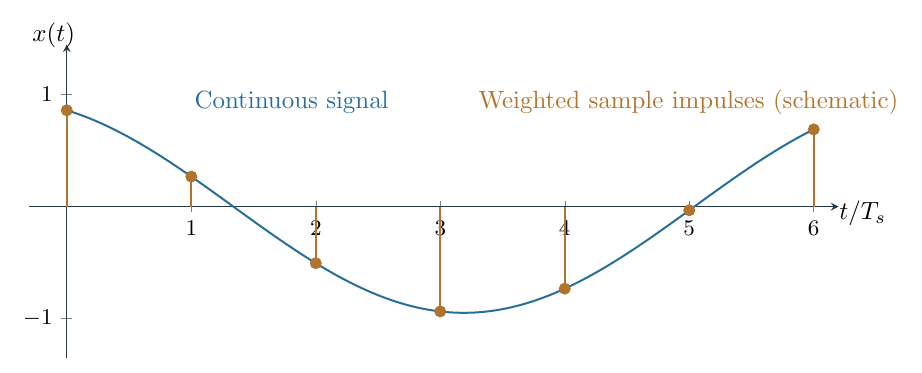
Figure 3. A continuous signal and schematic weighted impulses at uniformly spaced sampling
times. The stems depict the signed weights; the ideal delta impulses are mathematical
distributions, not finite-width rectangles.
6 Derive the Fourier transform of the impulse train
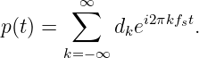
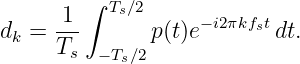
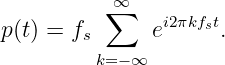
The impulse train has period Ts. This lets us reuse the complex Fourier series from FS18–FS20. Its
fundamental frequency is fs = 1∕Ts:
For a periodic generalized function, its coefficient over any period is
There is just one unit impulse in the interior of the selected period, at t = 0. Applying the sifting
identity,
| dk | =  e−i2πkfs(0) | (31)
|
| =  = fs. | (32) |
Thus every complex Fourier series coefficient of the ideal comb equals fs:
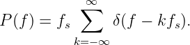
This equality is understood in the sense of distributions. Its value is that the Fourier transform of a
complex exponential is a frequency-domain delta:
Consequently,
A periodic impulse train in time transforms into a periodic impulse train in frequency. The spacing
in frequency is fs, the reciprocal of the spacing Ts in time.
7 Sampling replicates the Fourier spectrum
The Fourier-transform multiplication rule states that multiplication in time corresponds to
convolution in frequency:
Substitute the comb transform from Equation (35):
Distribute the convolution over the sum:
Convolution with a shifted delta shifts a function:
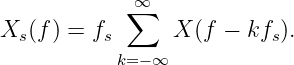
Therefore the sampled spectrum is
This is the central equation of the sampling theorem derivation.
Read the equation term by term
The term with k = 0 is the original spectrum X(f). The terms with k = 1 and k = −1 are copies
shifted right and left by fs. Higher integer values produce additional copies at 2fs, 3fs, and so on.
Every copy is multiplied by the factor fs.
This is the precise meaning of spectral replication. The sampling operation has not merely
discarded time samples. In the frequency representation of the impulse-sampled signal it has
created an infinite periodic family of translated spectra.
8 Derive the Nyquist sampling condition
Assume the original signal is band-limited to B:
Its unshifted support lies in the interval
The copy centered at fs occupies
To avoid overlap between the central support and the right-hand copy, require the central right
edge to lie to the left of the neighboring left edge:
Add B to both sides:
Hence
The left-hand neighboring copy gives the same result. The signal bandwidth 2B must fit within the
frequency separation fs between replicas.
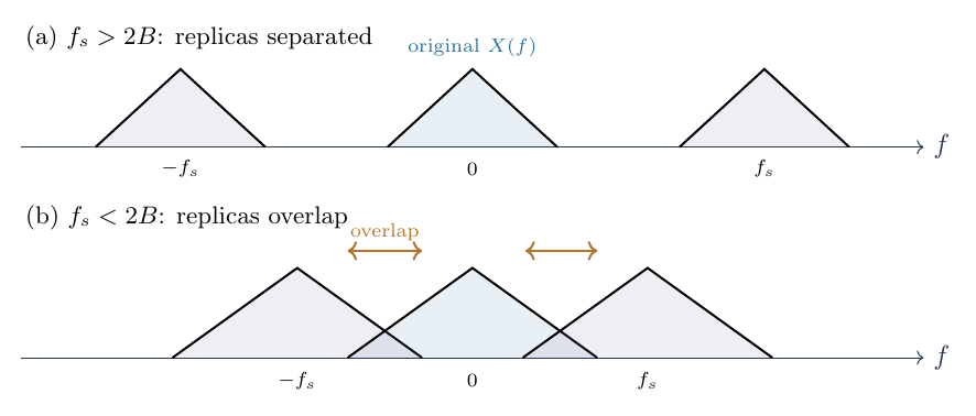
Figure 4. Schematic bilateral spectra. When the shift fs exceeds the original two-sided spectral
width 2B, the copies can be separated. When fs < 2B, neighboring copies overlap and their
contributions add irreversibly in the sampled spectrum.
The familiar statement “sample at twice the highest frequency” is the limiting boundary of this
spectral nonoverlap argument. In engineering practice one normally chooses a higher rate to allow
room for analog filtering and imperfections.
Why equality deserves care
At fs = 2B, neighboring supports touch at the band edge. For many mathematically well-behaved
L2 signals, isolated support endpoints are irrelevant to their integral representation. But a pure
sine precisely at fs∕2 illustrates a practical ambiguity:
Its sampled values are
for every integer n. A nonzero sinusoid has become indistinguishable from the zero sequence. Pure
eternal sinusoids are not finite-energy L2 signals, so this example does not contradict the usual
finite-energy theorem. It does show why a simple universal claim of guaranteed recovery
at the exact boundary is too strong without specifying the signal class and endpoint
assumptions.
9 Reconstruct the original spectrum with a filter
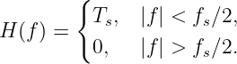
When fs > 2B, the spectral replicas are separated. We can isolate the central copy by an ideal
low-pass frequency response
The exact value at the cutoff boundary is immaterial for ordinary finite-energy signals, provided no
troublesome spectral line sits there.
Why is the passband gain Ts rather than one? Equation (40) shows that the impulse-sampled
spectrum has a multiplier fs = 1∕Ts. The reconstruction filter must cancel it:
Inside the baseband the output transform is therefore
Outside the baseband the shifted copies are suppressed. Taking the inverse transform recovers the
original signal.

Figure 5. An ideal low-pass response selects the isolated central spectrum and rejects its shifted
copies. The passband gain is Ts, which compensates for the fs factor in the impulse-sampled
spectrum.
The ideal filter is a mathematical reconstruction device. A real analog or digital reconstruction
chain has finite transition bands, latency, and nonideal behavior. It cannot perfectly implement an
infinitely sharp cutoff over all time.
10 Derive sinc interpolation, not just the sampling inequality
A stronger result is possible: the original time-domain function can be expressed directly in terms
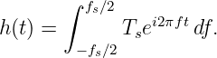
of its samples. Start from the ideal low-pass response in Equation (49). Its inverse Fourier
transform is the impulse response
For t≠0, integrate the exponential:
| h(t) | = Ts −fs∕2fs∕2 | (53)
|
| = Ts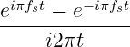 | (54)
|
| = Ts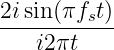 | (55)
|
| =  . | (56) |
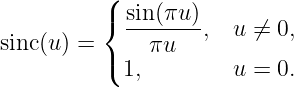
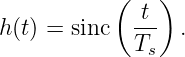
The last line uses Ts = 1∕fs. The continuous limit at t = 0 equals one. Define the normalized sinc
function by
Thus
The ideal reconstructed signal is the convolution of the impulse-sampled signal with this
response:
Insert the impulse representation from Equation (28) and use the sifting identity:
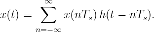
Therefore
This is the Whittaker-Shannon sinc interpolation formula.
Why the shifted sinc functions reproduce the samples
At another sample instant t = mTs, the sinc associated with sample n becomes
When m = n, its value is one. When m≠n, its argument is a nonzero integer and its value is zero.
Hence at t = mTs all sinc contributions vanish except the n = m contribution, which returns
x(mTs).
Between the sample instants all the shifted sinc functions overlap. Their weighted sum reconstructs
the continuous band-limited signal, not merely a set of isolated points.
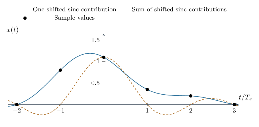
Figure 6. A finite illustrative sum of shifted sinc kernels. Each kernel contributes at intermediate
times, but at integer sample instants only its own sampled value survives. The displayed finite
combination is itself band-limited to the ideal Nyquist band.
The interpolation theorem is remarkable: knowledge of a band-limited continuous function at
infinitely many discrete, uniformly spaced times determines its values between those times. The
guarantee comes from the prior spectral restriction, not from the dots alone.
11 Why this is closely related to FS02 and FS11
FS02 introduced an inner product by weighting samples with Δt and letting the spacing shrink.
That produced integration over the time domain. This lecture uses a complementary idea: in
Fourier space, a periodic train imposes a frequency spacing, and its transform builds discrete copies
separated by fs.
FS11 interpreted a Fourier partial sum as projection onto a finite-dimensional span of orthogonal
functions. Here the signal is assumed to live in a restricted class of functions whose
spectra occupy a fixed band. The shifted sinc functions provide coordinates adapted to
regular samples: the sample values become the coefficients in the sinc reconstruction
formula.
An important distinction remains. A plot of a signal against time is not a picture of its abstract
function-space geometry. Sampling does not project a graph down onto isolated points. Rather, it
evaluates the signal at selected times. The band-limit assumption supplies the extra information
needed to infer what happened between those times.
12 A physics example: the spectrum of a force impulse
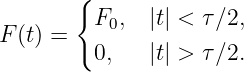
Suppose an external force acts on a mass with constant magnitude F0 for a short time τ centered
at t = 0:
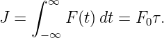
This idealized pulse can approximate a controlled thrust or mechanical contact force over a short
duration. The total impulse is
The impulse-momentum theorem then gives
for a particle when this is the net impulse. The Fourier transform reveals another aspect of the
same event.
Calculate its transform step by step
By definition,
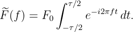
The force is nonzero only between −τ∕2 and τ∕2, so
For f≠0,
| F(f) | = F0 −τ∕2τ∕2 | (68)
|
| = F0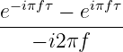 | (69)
|
| = F0 | (70)
|
| = F0τ sinc(fτ). | (71) |
Using J = F0τ gives
At zero frequency the limiting sinc value is one, so
This makes physical sense directly from the Fourier-transform definition: setting f = 0 removes the
oscillatory exponential, leaving the time integral of force, which is the impulse.
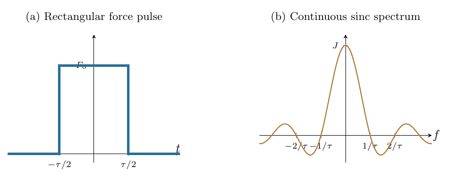
Figure 7. The transform of a finite rectangular force pulse is a sinc-shaped spectrum. Its value at
zero frequency is the total mechanical impulse J, and its first nonzero spectral zeros occur at
f = ±1∕τ.
Shorter in time means wider in frequency
The first nonzero zeros satisfy
so they occur at
If the pulse duration is halved, the first zeros move twice as far from the origin. The main spectral
lobe becomes broader. This is an elementary illustration of time-frequency localization, which will
be developed further in FS27.
For fixed total impulse J, shortening τ requires raising F0 = J∕τ. The zero-frequency transform
remains J, while the spectrum spreads outward. A sharper time-domain event demands a wider
range of Fourier frequencies.
Important limitation: the pulse is not band-limited
The sinc transform has side lobes extending to arbitrarily high frequencies. Therefore the ideal
rectangular force pulse is not strictly band-limited. No finite sampling rate satisfies the exact
hypotheses of the perfect-reconstruction theorem for this pulse without first modifying the
spectrum.
A real acquisition system must either accept some aliasing error or attenuate high-frequency
content with an analog anti-alias filter before sampling. The force-pulse example is still valuable
because it shows directly how narrowing a transient increases the bandwidth demanded of the
measurement system.
13 How an analog anti-alias filter differs from reconstruction
The sampling theorem involves two conceptually different filters.
- An anti-alias filter acts on the continuous analog signal before the sampler. It
attenuates frequency content that would fold into the selected sampled baseband.
- A reconstruction filter acts on the ideal impulse-sampled representation after sampling.
It selects the desired unshifted spectrum if the copies do not overlap.
If high-frequency spectral copies already overlap, a later digital low-pass filter cannot determine
which portion of the overlapping energy came from which original continuous-frequency band. The
information was lost in sampling.
An actual analog-to-digital converter also has finite aperture time, quantization, noise, jitter, and a
sample-and-hold response. These effects are separate from the basic ideal Nyquist argument and
may impose tighter design requirements.
14 Home electronics laboratory: see a 900 Hz tone become 100 Hz
A function generator with sine-wave output and a digitizer or oscilloscope capable of exporting
samples provides a direct experiment.

Figure 8. A bench experiment compares the continuous generator signal with the sampled record.
An optional analog low-pass filter demonstrates why high-frequency content must be rejected
before the analog-to-digital converter when it would alias.
Equipment and setup
Use a function generator, a digitizer with a known sampling frequency, and a means of plotting the
collected samples. A two-channel oscilloscope can be useful if one channel monitors the analog
signal while another view or exported file presents the sampled values. Choose a modest safe signal
amplitude compatible with the input range of the instrument. Follow the instrument’s grounding
and input-voltage instructions.
For clarity, select fs = 1000 samples∕s if the instrument permits this explicit rate. Some
oscilloscopes automatically change their sampling rate as the time-base setting changes; verify the
actual sample rate reported with the exported data.
First generate a 100 Hz sine or cosine, capture the samples, and plot them against sample index.
Then change the generator to 900 Hz while holding the sample rate constant. Compare the two
sampled sequences and their discrete Fourier transforms.
For equal-phase cosines, the ideal 100 Hz and 900 Hz sample sequences agree. For sine waves, a
phase or sign difference can arise when the high-frequency alias reflects through the Nyquist
boundary. Distinct continuous signals can still generate indistinguishable or predictably related
sampled sequences.
Numerical predictions before connecting hardware
For fs = 1000 Hz, the Nyquist frequency is 500 Hz. The following positive-tone examples have the
stated real-cosine aliases:
| Input tone (Hz) | Selected integer k | Alias magnitude (Hz) |
|
|
|
| 100 | 0 | 100 |
| 400 | 0 | 400 |
| 600 | 1 | 400 |
| 900 | 1 | 100 |
| 1200 | 1 | 200 |
The table is a prediction for ideal uniform sampling. The FFT of a finite record adds issues of
windowing, frequency-bin resolution, and leakage, but the alias locations themselves follow from
the sampling geometry.
Optional filter demonstration
Insert a suitably designed analog low-pass filter between the generator and the digitizer. Its cutoff
and transition band should substantially attenuate the 900 Hz input while preserving the 100 Hz
component. The 900 Hz alias should then decrease in the sampled record. Applying the same
low-pass filter after the 900 Hz input has already been sampled cannot restore its missing
original-frequency identity.
15 Checks that prevent common mistakes
Check 1: sampling frequency versus Nyquist frequency
fs is the number of samples per second. The Nyquist frequency is fs∕2. Confusing these quantities
introduces a factor-of-two error. A 1000 samples/s system has Nyquist frequency 500 Hz, not 1000
Hz.
Check 2: a signal must be restricted in frequency
Uniform samples do not uniquely determine an arbitrary continuous function. Infinitely many
non-band-limited functions can agree at every sampling time. The band-limit assumption removes
that ambiguity within the specified signal class.
Check 3: the reconstruction filter must remove the comb scaling
The ideal impulse train used here has unit impulse area at every sampling time. Its Fourier
transform carries a factor fs. The corresponding ideal reconstruction response has passband gain
Ts. A different impulse-train normalization would change both factors but not the underlying
reconstruction theorem.
Check 4: frequency units and transform conventions
The convention in Equation (1) uses hertz and e−i2πft. If instead the transform is defined using
angular frequency ω, the Nyquist angular frequency is
while ωs = 2π∕Ts. Do not mix f and ω within the same transform without converting the factors
of 2π.
16 Worked mini-exercises with solutions
Exercise A: determine the sampling period
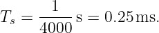
A sensor reports 4000 measurements each second. Find Ts and fN.
Solution. From Equation (3),
The Nyquist frequency is
Exercise B: alias a higher-frequency tone
A 740 Hz cosine is sampled at 1000 samples∕s. Predict its baseband alias.
Solution. Shift by one sampling frequency:
The sampled cosine is indistinguishable from a 260 Hz cosine with the appropriate phase
convention.
Exercise C: calculate a minimum strict sampling rate
A real signal has no Fourier content outside [−1800, 1800] Hz. What nonoverlap inequality should
the sample rate satisfy?
Solution. The two-sided spectral width is 3600 Hz. Require
The nominal Nyquist rate is 3600 samples/s, but a practical system needs additional
margin.
Exercise D: pulse duration and spectrum
A rectangular force pulse lasts 2 ms and delivers 0.6 N s of impulse. Find F0 and its first positive
spectral zero.
Solution. The force magnitude is
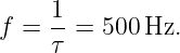
The first positive spectral zero occurs at
This does not mean that the pulse has no energy above 500 Hz. It has infinitely extended sinc side
lobes.
Exercise E: distinguish samples from the analog waveform
Can a low-pass filter applied to samples from a 900 Hz cosine taken at 1000 samples/s recover the
original 900 Hz tone uniquely?
Solution. No. The same samples could have come from a 100 Hz cosine. A digital filter acting only
on that sequence cannot determine which analog waveform was present. The measurement chain
must constrain the analog bandwidth before sampling.
17 Summary and bridge to further Fourier analysis
The essential chain of reasoning is now complete:
- Sampling a sinusoid introduces frequency ambiguity modulo the sample rate.
- Ideal sampling by a Dirac comb replicates the entire Fourier spectrum at frequency
offsets kfs.
- If a signal occupies only [−B,B], separation of neighboring spectral copies requires
fs > 2B in the strict nonoverlap form.
- A properly scaled ideal low-pass filter selects the unshifted spectrum when the replicas
do not overlap.
- The inverse transform of that ideal filter is a sinc function, yielding exact shifted-sinc
interpolation under the theorem’s assumptions.
- A short physical impulse has a broad spectrum and is not itself strictly band-limited;
acquisition systems must handle out-of-band content before digitization.
This lecture makes the connection from Fourier series to Fourier transforms physically tangible. It
also prepares for FS27, where wave packets, localization, and dispersion make the relationship
between time extent and spectral width central to the physics.
References
[1] C. E. Shannon, “Communication in the Presence of Noise,” Proceedings of the IRE,
37, 10–21 (1949).
[2] A. V. Oppenheim and R. W. Schafer, Discrete-Time Signal Processing, 3rd ed.
(Pearson, 2010).
[3] R. N. Bracewell, The Fourier Transform and Its Applications, 3rd ed. (McGraw-Hill,
2000).