Strapdown Inertial Navigation: Attitude Kinematics from Gyroscope Measurements
A strapdown inertial navigation system has no mechanically stabilized platform. The inertial
sensors rotate with the vehicle, so the navigation computer must continuously reconstruct the
orientation of the body frame from gyroscope measurements. This reconstruction is the attitude
mechanization.
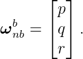
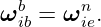
The physical input is the inertial body angular rate measured by the gyro triad,
For navigation relative to the local NED frame, this is not yet the rate that should drive the
attitude solution. INS06 showed that the navigation frame itself rotates relative to inertial space
with
Therefore the body rate relative to NED is
This one physical angular-rate vector can drive several mathematical attitude representations. Four
are especially important in inertial navigation:
- the direction cosine matrix (DCM);
- three Euler Angles;
- a unit quaternion;
- a finite rotation vector.
They do not describe four different attitudes. They are four coordinate descriptions of the same
element of the three-dimensional rotation group SO(3) [1, 2, 3, 4].
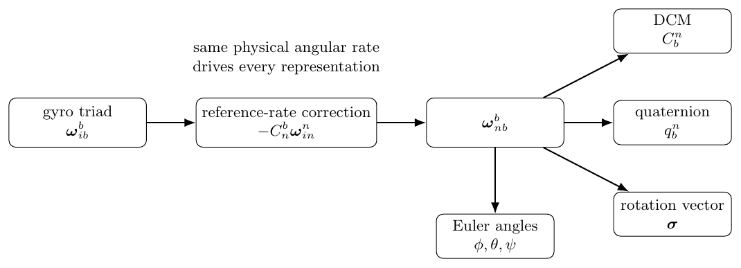
Figure. The gyroscope measures inertial body rate. After navigation-frame rotation is
removed, the same relative angular rate ωnbb can propagate a DCM, Euler angles, a
quaternion, or a rotation vector.
1 Learning objectives
After completing this entry, the reader should be able to:
- explain why a gyroscope measures angular rate rather than attitude;
- convert the gyro measurement ωibb into the body rate relative to NED;
- derive the continuous DCM attitude equation;
- derive the 3-2-1 Euler-angle rate equations from the body angular-rate vector;
- identify the Euler-angle singularity at pitch 𝜃 = ±90∘;
- define a scalar-first Hamilton quaternion that represents Cbn;
- derive quaternion kinematics from the same body-relative angular rate;
- construct an exact finite quaternion increment from an angular increment;
- relate the matrix exponential, Rodrigues formula, and a finite rotation vector;
- state the Bortz rotation-vector differential equation and its small-angle form;
- compare the numerical advantages and disadvantages of DCM, Euler-angle, quaternion,
and rotation-vector propagation;
- formulate practical invariants and unit tests for an attitude mechanization.
2 The attitude problem is a kinematic problem
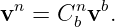
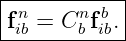
Let Cbn transform body-resolved vector components into navigation-frame components,
At one instant, Cbn answers the geometric question: how are the body axes oriented relative to the
navigation axes? The gyroscope answers a different question: how rapidly is that orientation
changing?
The attitude mechanization must therefore integrate angular velocity on the geometry of
rotations.
For scalar translation, integrating velocity is straightforward because ordinary vector addition
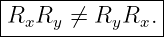
commutes. Three-dimensional rotations are different. If Rx and Ry are finite rotations about two
different axes, then in general
This noncommutativity is why three gyro channels cannot generally be integrated as three
independent scalar angles.
3 From gyro rate to navigation-relative body rate
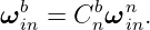
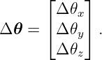
The ideal gyro triad supplies
The local navigation frame has inertial angular rate
Resolved in body coordinates,
Angular velocities add according to their frame relationships,
Thus
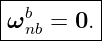
A stationary vehicle fixed to Earth is an important limiting case. If the body remains aligned with
NED, then
and therefore
The gyro can measure Earth rate while the Earth-relative attitude remains constant.
4 Direction cosine matrix kinematics
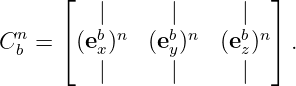
The DCM is the most direct representation of the coordinate transformation itself. Its columns are
the body basis vectors resolved in navigation coordinates.
Let
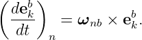
Each body basis vector rotates relative to the navigation frame according to
Resolve the angular rate in body coordinates. Using the skew-symmetric cross-product matrix
introduced in INS01,
collecting the three differentiated columns gives
This is the relative-rate form of the DCM attitude equation.
4.1 Recovering the full strapdown equation
Insert
Then
 | = Cbn[ω
ibb]
×− Cbn[C
nbω
inn]
×. | (18) |
The cross-product transformation identity is
Therefore
Using INS06,
The first term rotates the body relative to inertial space. The second term removes the rotation of
the navigation frame itself.
5 Finite DCM propagation
Suppose the corrected body-relative angular rate is approximately constant over a short interval
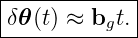
Δt. Define the body-resolved angular increment
The DCM differential equation then has the finite solution
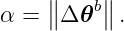
The matrix exponential is a true finite rotation. Let
Rodrigues’ formula gives
For small α,
The second-order term is important because I + [Δ𝜃]× is not exactly orthogonal.
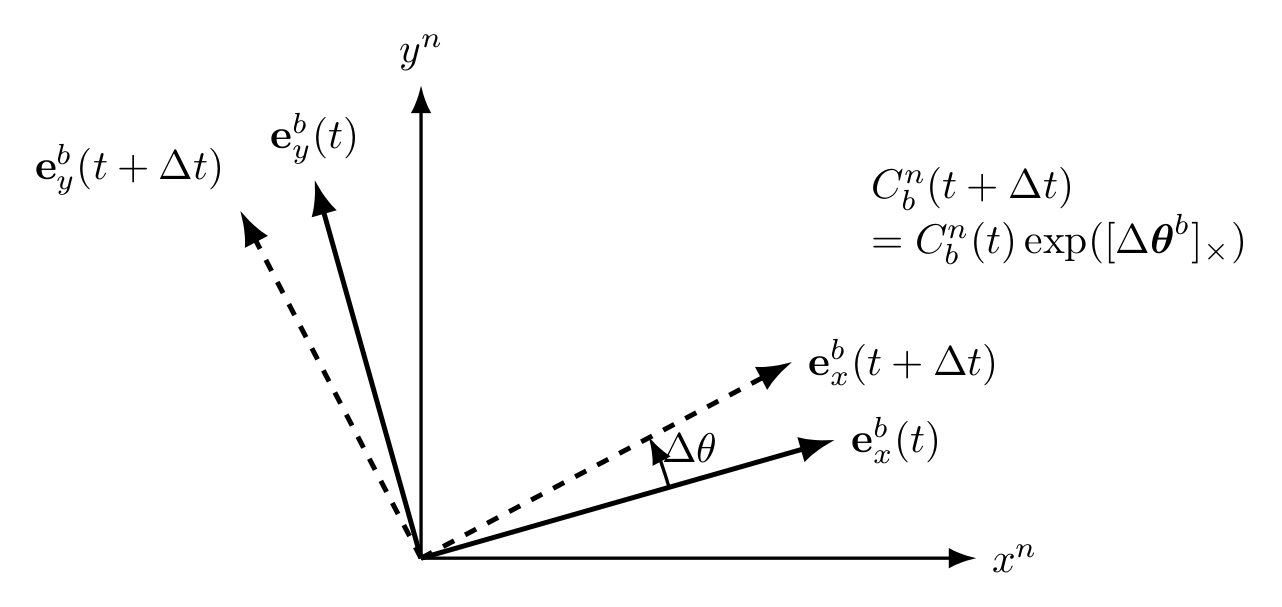
Figure. A finite angular increment rotates the body basis from its orientation at sample k
to the orientation at sample k + 1. The exponential map keeps the update on the rotation
group SO(3).
5.1 A two-sided update using raw gyro rate
If the inertial body increment and navigation-frame increment are handled separately, a useful
short-interval form is
This form makes the physics visible. The body is advanced by the gyro-measured inertial rotation
on the right, while the navigation axes are advanced on the left. Higher-order algorithms refine how
the two increments are formed within the sample interval [4].
6 Euler angles: a minimal but singular description
Euler angles use only three numbers. For navigation, a common convention is the 3-2-1
yaw-pitch-roll sequence
The attitude matrix may be written
using the passive DCM convention of INS01.
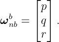
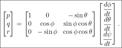
Let the body rate relative to NED, resolved in body coordinates, be
The three Euler-angle rates do not equal p, q, and r. Each elemental Euler rotation is taken about
a different intermediate axis.
6.1 Deriving the Euler-rate mapping
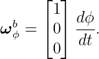
The roll contribution is already about the final body x axis,
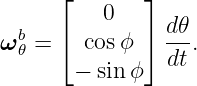
The pitch rotation, after the roll rotation is accounted for, resolves in body axes as
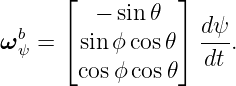
The yaw contribution resolves as
Adding the three contributions gives
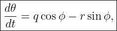
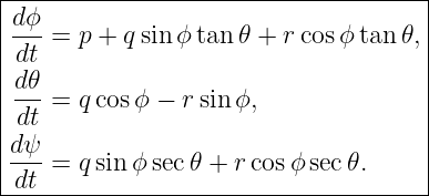
Inverting the matrix gives the familiar 3-2-1 Euler kinematics,
and
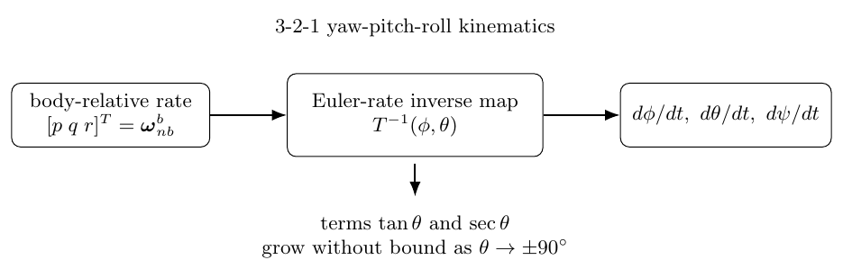
Figure. Euler-angle rates are obtained through a state-dependent kinematic map. The
factors tan 𝜃 and sec 𝜃 reveal the 3-2-1 singularity at pitch 𝜃 = ±90∘.
6.2 The Euler-angle singularity
As
both tan 𝜃 and sec 𝜃 become unbounded. The physical attitude and angular velocity remain
perfectly finite. It is the coordinate description that becomes singular.
This is often called gimbal lock. It is a representation singularity, not a failure of rigid-body
mechanics.
Euler angles remain valuable for display, interpretation, and moderate-angle applications.
They are usually a poor choice for the internal attitude state of a general strapdown
navigator.
7 Quaternion attitude representation
A unit quaternion represents attitude with four numbers and one norm constraint. In this article a
scalar-first Hamilton quaternion is written
The quaternion represents the same body-to-navigation transformation as Cbn.
One DCM consistent with this convention is
The signs in quaternion formulas depend on whether a text uses active or passive rotations,
scalar-first or scalar-last storage, and Hamilton or alternate multiplication conventions. A
navigation implementation should state its convention explicitly and test it against a known
one-axis rotation.
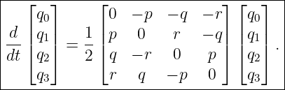
8 Quaternion differential equation
Form a pure-vector quaternion from the body-relative angular rate,
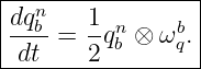
For the convention above, quaternion kinematics are
Let
Then
The 4 × 4 rate matrix is skew-symmetric. Therefore the exact continuous dynamics preserve unit
norm.
Indeed,
 (qT q) (qT q) | = 2qT  | (45)
|
| = qT Ω(ω)q | (46)
|
| = 0. | (47) |
Numerical integration can still cause small norm drift, so practical implementations often
renormalize after each update.
8.1 Using the raw gyro and navigation rates separately
The relative-rate equation can also be written directly in terms of the gyro measurement and
navigation-frame inertial rate,
This is the quaternion analogue of the two-term DCM equation.
9 Finite quaternion propagation
Suppose a corrected angular increment over one IMU interval is
Define
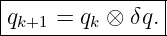
The exact unit quaternion for that finite rotation is
The attitude update is
For very small α,
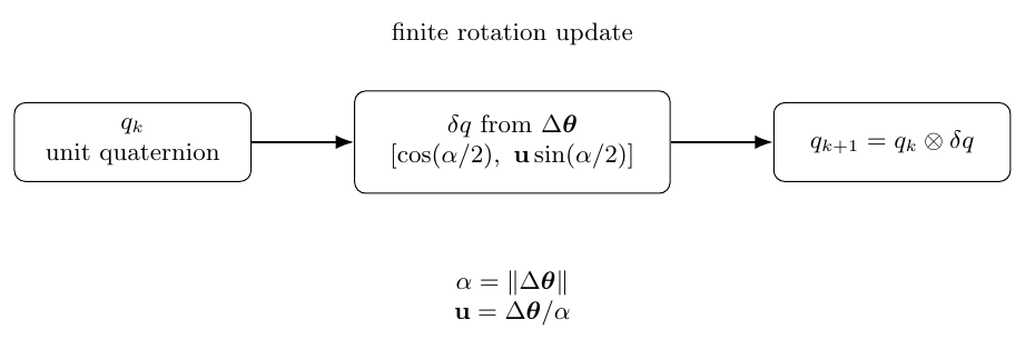
Figure. A finite angular increment can be converted directly into an incremental unit
quaternion. Quaternion multiplication composes the old attitude with the new finite
rotation.
10 Rotation vectors and the exponential map
A finite rotation may also be represented by a three-component rotation vector
where u is the rotation axis and α is the rotation angle.
The corresponding DCM increment is
Because
its exponential series can be regrouped into Rodrigues’ formula,
Thus the rotation vector, DCM exponential, and incremental quaternion are three descriptions of
the same finite rotation.
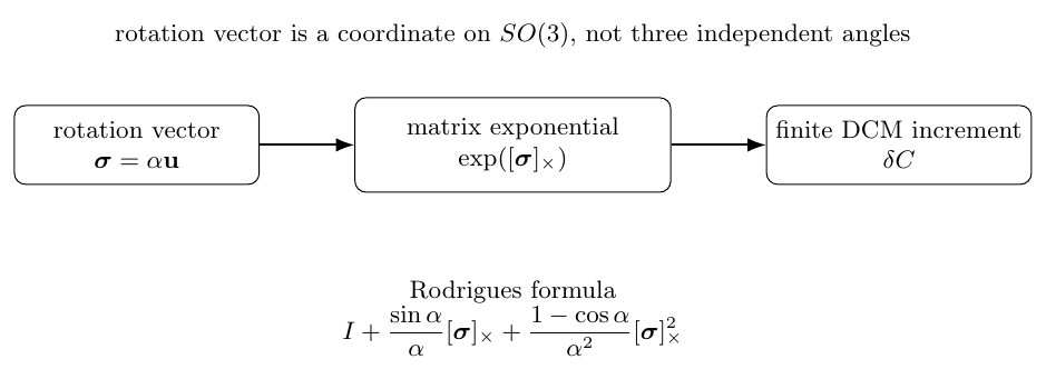
Figure. The rotation vector carries an axis in its direction and a rotation angle in its
magnitude. The exponential map converts that three-component coordinate into a finite
DCM increment.
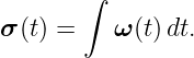
11 Why the rotation vector is not simply the integral of angular rate
If the angular velocity keeps a constant direction, then the finite rotation vector is simply
For general three-dimensional motion, the direction of the angular rate changes, finite rotations do
not commute, and the relationship is more complicated.
For the convention
Bortz’s rotation-vector equation may be written [5, 4]
where
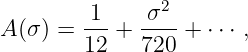
For small rotation vectors,
so
The cross-product terms are the beginning of the finite-rotation corrections that later lead to
coning algorithms.
12 One physical maneuver in four representations
Consider a body already aligned with NED. After reference-frame correction, suppose the body
rotates about its down axis at
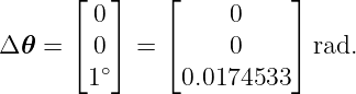
for
Then
12.1 Euler-angle view
At zero roll and pitch,
so
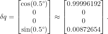
12.2 Quaternion view
The incremental quaternion is
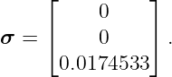
12.3 Rotation-vector view
The increment is simply
12.4 DCM view
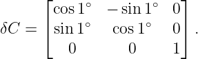
Rodrigues’ formula gives
All four descriptions represent the same physical one-degree yaw rotation.
13 Why forward Euler integration damages a DCM
A tempting discrete approximation is
Let
Even if CkT C
k = I,
| Ck+1T C
k+1 | ≈ (I + S)T (I + S) | (74)
|
| = (I − S)(I + S) | (75)
|
| = I − S2. | (76) |
The error is second order in the angular increment but accumulates over time. A finite exponential
update stays orthogonal by construction.
This provides a general numerical lesson:
14 Quaternion normalization and finite increments
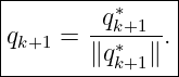
A first-order quaternion integration step has the form
The new vector qk+1∗ will generally not have exactly unit norm in finite-precision arithmetic. A
common correction is
Using an exact incremental quaternion is usually preferable when a finite angular increment is
already available from the IMU.
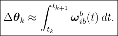
15 Gyro angular increments rather than continuous rates
A real digital IMU commonly reports either an angular rate sampled over a finite interval or an
integrated angular increment
This makes finite rotation updates natural. However, a simple componentwise integral does not
capture every effect of a changing rotation axis within the interval. The noncommutative
corrections required for high-dynamic motion are called coning corrections. They will be developed
later from the same rotation-vector structure introduced here.
16 Representation comparison
|
|
|
|
|
| Representation | States | Constraint | Global singularity | Typical INS use |
|
|
|
|
|
| DCM | 9 | CT C = I, det C = 1 | none | direct geometry, checks |
| Euler angles | 3 | none | yes | display, interpretation |
| Quaternion | 4 | qT q = 1 | none | primary propagation |
| Rotation vector | 3 | local coordinate | log-map ambiguity | increments, corrections |
|
|
|
|
|
The phrase “no singularity” for a quaternion means there is no attitude singularity analogous to
Euler gimbal lock. Quaternions have the double-cover property
representing the same physical attitude.
A finite rotation vector is also not globally unique. Axis-angle representations repeat after full
turns, and the principal logarithm becomes ambiguous for rotations near 180∘. In strapdown
algorithms, rotation vectors are therefore especially useful as local finite increments rather than as
an unrestricted global attitude coordinate.
17 A stationary-Earth consistency test
One of the strongest attitude-mechanization unit tests uses a body fixed to Earth.
Suppose
Then
The ideal gyro measures
The reference-rate correction yields
| ωnbb | = ω
ibb − C
nbω
ien | (85)
|
| = 0. | (86) |
Every representation must therefore remain constant:
If a stationary Earth-fixed simulated IMU causes attitude to rotate at approximately Earth rate,
the navigation-frame correction is missing or has the wrong sign.
18 Gyro bias and attitude drift
Let the measured gyro rate contain a small constant bias,
Over a short interval in which the frame geometry can be treated as fixed, the corresponding small
attitude error grows approximately as
This is the rotational analogue of integrating an accelerometer bias into velocity error.
The consequences are even more severe because attitude error rotates gravity into the
horizontal acceleration channels. INS19 will derive the resulting coupled navigation error
dynamics.
19 Implementation checks
A robust attitude implementation should contain invariants that can be checked automatically.
19.1 DCM checks
Verify
A determinant near one by itself is not enough. Orthogonality must also be checked.
19.2 Quaternion checks
Verify
and confirm
when quaternion and DCM propagators are run in parallel.
19.3 One-axis exact solution
For constant rate r about the down axis,
has an exact closed-form solution. DCM, quaternion, Euler-angle, and rotation-vector
implementations should all reproduce it.
19.4 Stationary Earth-fixed solution
After Earth-rate correction, a body fixed to the local NED frame should have zero relative angular
rate and constant attitude.
19.5 Round-trip coordinate transformations
For nonsingular attitudes, convert
and
The reconstructed DCM should agree with the original to numerical precision.
20 Connection to the rest of the strapdown mechanization
Attitude is not an isolated output. The accelerometers measure specific force in body
coordinates,
The attitude solution supplies the transformation
The transformed specific force then enters the NED velocity equation,
An attitude error is therefore immediately an acceleration error. This is why attitude propagation
is the first major numerical operation performed on each new gyro sample.
21 Connection to subsequent INS lessons
INS08 will deepen the quaternion and finite-increment treatment, with special attention to discrete
propagation and numerical implementation.
INS09 will use gravity and Earth rate as reference vectors for initial attitude alignment.
INS15 will place the attitude propagator inside the complete NED attitude, velocity, and position
mechanization.
INS16 and INS17 will move from ideal continuous rates to sampled IMU increments, including
finite-rotation, coning, and sculling corrections.
INS18 and INS19 will introduce sensor errors and derive the resulting attitude and navigation error
dynamics.
22 Summary
The gyro measures
while local-level attitude propagation requires
The DCM equation is
For 3-2-1 Euler angles,
For the scalar-first Hamilton quaternion convention used here,
A finite rotation vector produces the DCM increment
and the equivalent quaternion increment
The representation changes, but the underlying physics does not. The navigation computer is
integrating one angular-velocity vector on the geometry of three-dimensional rotations.
References
[1] David H. Titterton and John L. Weston, Strapdown Inertial Navigation Technology,
2nd ed., Institution of Electrical Engineers, 2004.
[2] Paul D. Groves, Principles of GNSS, Inertial, and Multisensor Integrated Navigation
Systems, 2nd ed., Artech House, 2013.
[3] Christopher Jekeli, Inertial Navigation Systems with Geodetic Applications, Walter
de Gruyter, 2001.
[4] Paul G. Savage, “Strapdown Inertial Navigation Integration Algorithm Design Part
1: Attitude Algorithms,” Journal of Guidance, Control, and Dynamics, vol. 21, no. 1,
pp. 19–28, 1998.
[5] John E. Bortz, “A New Mathematical Formulation for Strapdown Inertial
Navigation,” IEEE Transactions on Aerospace and Electronic Systems, vol. AES-7, no.
1, pp. 61–66, 1971.









![[a]×b = a × b,](https://images.physicslibrary.org/cache/objects/1356/make4ht/StrapdownInertialNavigationAttitudeKinematicsFromGyroscopeMeasurements14x.png)
![|------------------|
|dCnb- n b |
| dt = Cb [ω nb]×.|
-------------------](https://images.physicslibrary.org/cache/objects/1356/make4ht/StrapdownInertialNavigationAttitudeKinematicsFromGyroscopeMeasurements15x.png)

![Cn [Cb an]× = [an]×Cn .
b n b](https://images.physicslibrary.org/cache/objects/1356/make4ht/StrapdownInertialNavigationAttitudeKinematicsFromGyroscopeMeasurements18x.png)
![|----------------------------|
|dCnb- n b n n |
| dt = C b [ω ib]× − [ω in]×C b .
------------------------------](https://images.physicslibrary.org/cache/objects/1356/make4ht/StrapdownInertialNavigationAttitudeKinematicsFromGyroscopeMeasurements19x.png)
![|---n------------------------------|
|dCb--= Cn [ωb ] − [ωn + ωn ] Cn .|
--dt------b--ib×------ie----en-×--b--](https://images.physicslibrary.org/cache/objects/1356/make4ht/StrapdownInertialNavigationAttitudeKinematicsFromGyroscopeMeasurements20x.png)

![|--------------------------|
Cn = Cn exp ([Δ 𝜃b]× ).|
--b,k+1-----b,k---------------](https://images.physicslibrary.org/cache/objects/1356/make4ht/StrapdownInertialNavigationAttitudeKinematicsFromGyroscopeMeasurements22x.png)
![|------------------------------------------------|
| sin α 1 − cosα |
|exp ([Δ 𝜃]×) = I + -----[Δ 𝜃]× + -----2---[Δ𝜃 ]2×. |
---------------------α--------------α------------](https://images.physicslibrary.org/cache/objects/1356/make4ht/StrapdownInertialNavigationAttitudeKinematicsFromGyroscopeMeasurements24x.png)
![exp ([Δ 𝜃]×) ≈ I + [Δ 𝜃]× + 1[Δ 𝜃]2.
2 ×](https://images.physicslibrary.org/cache/objects/1356/make4ht/StrapdownInertialNavigationAttitudeKinematicsFromGyroscopeMeasurements25x.png)
![--------------------------------------------
| n n n ( b ) |
-Cb,k+1-≈-exp-(−-[Δ-𝜃-in]×)-Cb,k-exp-[Δ-𝜃ib]×--.-](https://images.physicslibrary.org/cache/objects/1356/make4ht/StrapdownInertialNavigationAttitudeKinematicsFromGyroscopeMeasurements26x.png)





![|-----⌊--⌋---------------------------|
| q0 [ ] |
| n ||q1|| q0 n T n |
|qb = ⌈q2⌉ = qv , (qb) qb = 1.|
| q |
--------3-----------------------------](https://images.physicslibrary.org/cache/objects/1356/make4ht/StrapdownInertialNavigationAttitudeKinematicsFromGyroscopeMeasurements38x.png)

![[ 0 ]
ωbq = b .
ω nb](https://images.physicslibrary.org/cache/objects/1356/make4ht/StrapdownInertialNavigationAttitudeKinematicsFromGyroscopeMeasurements40x.png)
![|------------[----]-----[---]-------|
dqnb 1- n 0 1- 0 n |
|dt = 2 qb ⊗ ωb − 2 ωn ⊗ qb. |
----------------ib---------in---------](https://images.physicslibrary.org/cache/objects/1356/make4ht/StrapdownInertialNavigationAttitudeKinematicsFromGyroscopeMeasurements46x.png)

![|-------------------|
| [ ] |
δq = cos(α ∕2) . |
| u sin(α ∕2) |
---------------------](https://images.physicslibrary.org/cache/objects/1356/make4ht/StrapdownInertialNavigationAttitudeKinematicsFromGyroscopeMeasurements49x.png)
![[ 2 ]
δq ≈ 1 − α ∕8 .
Δ 𝜃∕2](https://images.physicslibrary.org/cache/objects/1356/make4ht/StrapdownInertialNavigationAttitudeKinematicsFromGyroscopeMeasurements51x.png)

![|----------------|
-δC-=--exp([σ-]×).-](https://images.physicslibrary.org/cache/objects/1356/make4ht/StrapdownInertialNavigationAttitudeKinematicsFromGyroscopeMeasurements53x.png)
![[σ ]3× = − α2[σ ]×,](https://images.physicslibrary.org/cache/objects/1356/make4ht/StrapdownInertialNavigationAttitudeKinematicsFromGyroscopeMeasurements54x.png)
![|------------------------------------|
| sin-α- 1 −-cosα- 2 |
|δC = I + α [σ ]× + α2 [σ ]×.|
--------------------------------------](https://images.physicslibrary.org/cache/objects/1356/make4ht/StrapdownInertialNavigationAttitudeKinematicsFromGyroscopeMeasurements55x.png)
![C = exp([σ ]× ), dC- = C [ω]×,
dt](https://images.physicslibrary.org/cache/objects/1356/make4ht/StrapdownInertialNavigationAttitudeKinematicsFromGyroscopeMeasurements57x.png)

![|------------------------------------------|
| 1--[ σ- ( σ) ] |
|A(σ ) = σ2 1 − 2 cot 2 , σ = ∥σ ∥.|
--------------------------------------------](https://images.physicslibrary.org/cache/objects/1356/make4ht/StrapdownInertialNavigationAttitudeKinematicsFromGyroscopeMeasurements59x.png)





![Ck+1 ≈ Ck (I + [ωΔt ]×).](https://images.physicslibrary.org/cache/objects/1356/make4ht/StrapdownInertialNavigationAttitudeKinematicsFromGyroscopeMeasurements70x.png)
![T
S = [ω Δt ]×, S = − S.](https://images.physicslibrary.org/cache/objects/1356/make4ht/StrapdownInertialNavigationAttitudeKinematicsFromGyroscopeMeasurements71x.png)

















![|----------------------------------------|
|dCnb n b n b n n |
|-dt--= C b [ω nb]× = C b [ω ib]× − [ω in]×C b .
------------------------------------------](https://images.physicslibrary.org/cache/objects/1356/make4ht/StrapdownInertialNavigationAttitudeKinematicsFromGyroscopeMeasurements94x.png)
![|-------------[----]-|
|dqnb 1 n 0 |
|----= -qb ⊗ ωb .|
-dt-----2--------nb---](https://images.physicslibrary.org/cache/objects/1356/make4ht/StrapdownInertialNavigationAttitudeKinematicsFromGyroscopeMeasurements96x.png)
![|----------------|
|δC = exp([σ ]×),|
------------------](https://images.physicslibrary.org/cache/objects/1356/make4ht/StrapdownInertialNavigationAttitudeKinematicsFromGyroscopeMeasurements97x.png)
![|-----[---------------]--|
| cos(σ ∕2) |
|δq = .|
| (σ ∕σ )sin (σ ∕2) |
-------------------------](https://images.physicslibrary.org/cache/objects/1356/make4ht/StrapdownInertialNavigationAttitudeKinematicsFromGyroscopeMeasurements98x.png)