Celestial Mechanics: Newton’s Equation for Orbital Motion
CM01 introduced Newton’s law of universal gravitation as a force law. CM02 then expressed the
same interaction through gravitational potential and potential energy. CM03 now turns that
physics into a dynamical equation: given an object’s position and velocity now, how does gravity
determine its future motion?
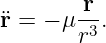
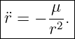
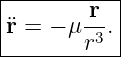
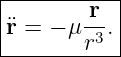
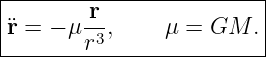
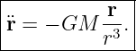
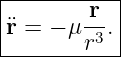
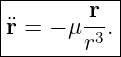
For a particle moving in the gravity of a spherical body of mass M, the central result
is
This equation is the Newtonian point-mass equation of orbital motion. It is a second-order
vector differential equation. Nearly everything developed later in elementary celestial
mechanics—orbital energy, angular momentum, conic sections, Kepler’s laws, orbital elements, and
time-of-flight relations—will follow from this equation plus suitable initial conditions
[1, 2, 3, 4, 5].
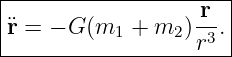
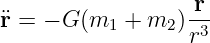
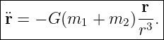
A second important result is that for two finite masses m1 and m2, the exact relative coordinate
obeys
Thus the same mathematical form appears again, but with gravitational parameter
The derivation of these equations is the main goal of CM03.
1 From gravitational force to acceleration
Place a spherical gravitating body of mass M at the origin. Let a particle of mass m have position
vector
with magnitude
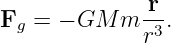
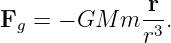
Newton’s gravitational force on the particle is
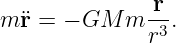
Newton’s second law is
Because acceleration is the second time derivative of position,
Therefore
Cancel the particle mass m:
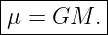
Define the gravitational parameter
Then the orbital equation becomes
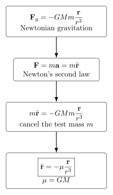
Figure. Newton’s orbital equation follows directly by combining universal gravitation with
Newton’s second law. The orbiting particle’s mass cancels, leaving the source gravitational
parameter μ = GM.
2 Why the test mass cancels
The gravitational force is proportional to the orbiting mass:
But the inertial resistance to acceleration in Newton’s second law is also proportional to that same
mass:
Therefore
contains no remaining factor of the test mass. In Newtonian theory, two sufficiently
small test bodies released from the same position with the same initial velocity follow
the same trajectory in a prescribed gravitational field, independent of their individual
masses.
This cancellation is the orbital-motion version of the result already encountered in CM01:
The source mass determines the field; the test particle responds to that field.
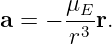
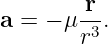
3 Why the vector equation contains r∕r3
The scalar inverse-square magnitude is
But an equation of motion must specify direction as well as magnitude. The inward radial unit
vector is
Since
we can write
| a | = − r r | (20)
|
| = −  | (21)
|
| = −μ . . | (22) |
Thus the apparently unusual denominator r3 is simply the combination of
for the force magnitude and
for the radial direction.
4 The minus sign means central attraction
The vector r points from the source at the origin toward the orbiting particle. Gravity points in
the opposite direction, back toward the source. Hence
The acceleration is therefore always antiparallel to r:
This does not mean the velocity must point inward. In orbital motion the velocity often has a large
transverse component. Gravity continuously bends the trajectory because the velocity and
acceleration generally point in different directions.
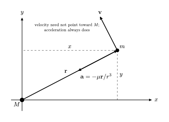
Figure. At an arbitrary point on an orbit, velocity can point in a direction quite different
from the gravitational acceleration. The acceleration always points toward the attracting
center, while the velocity is tangent to the instantaneous trajectory.
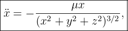
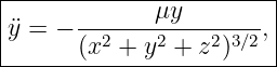
5 Cartesian component equations
Because
we have
Substitute into the orbital equation:
Matching components gives
and
These three coupled scalar differential equations are exactly equivalent to the compact vector
equation.
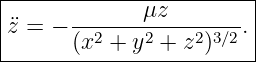
6 A dimensional check
The gravitational parameter has units
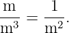
The factor
has dimensions
Therefore
which is the correct dimension for acceleration.
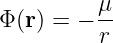
7 Connection with gravitational potential
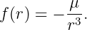
CM02 derived
for a point or spherically symmetric source outside its mass distribution, together with
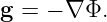
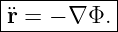
Since a freely moving test body has
we can also write the equation of motion as
For
this becomes
Thus the force-law, field, and potential descriptions all lead to the same dynamics.
8 The equation is a differential equation, not an orbit formula
The expression
specifies acceleration at each position. It does not yet tell us directly whether the resulting
trajectory will be a circle, ellipse, parabola, or hyperbola.
To obtain a unique trajectory, we must also specify an initial position and initial velocity:
The pair (r0,v0) determines the particular solution of the orbital differential equation.
Different initial velocities at the same position can produce completely different trajectories even
though the gravitational law is identical.
9 First-order state form
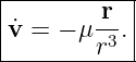
Numerical mechanics usually rewrites the second-order equation as two coupled first-order vector
equations. Define
Then
and
Define the six-component state
Then
This is the form that will later be integrated numerically.
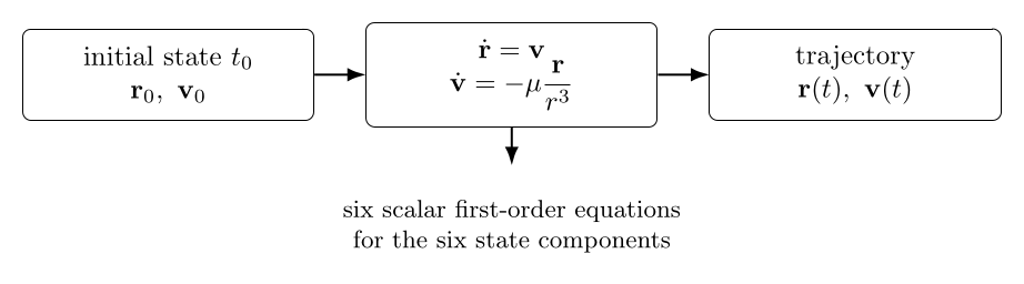
Figure. The orbital problem is an initial-value problem. Position and velocity at one time,
together with the differential equations, determine the subsequent Newtonian trajectory.
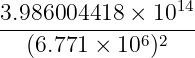
10 Example 1: gravitational acceleration at 400 km altitude
Take Earth’s gravitational parameter as
Use mean Earth radius
At altitude
the geocentric distance is
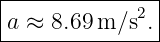
The acceleration magnitude is
| a | =  | (54)
|
| =  | (55)
|
| ≈ 8.69 m/s2. | (56) |
Thus
A spacecraft in low Earth orbit is therefore not in a region where gravity is nearly absent. Its
orbital motion is continuous free fall under a gravitational acceleration still close to terrestrial
surface gravity.
11 Example 2: evaluate the acceleration vector
Suppose a spacecraft has geocentric position
Convert to meters:
The radius is
| r | =  | (60)
|
| ≈ 7.280 × 10⁶ m. | (61) |
The acceleration is
Using the numerical values gives approximately
Its magnitude is about
consistent with
The component signs are not arbitrary: both are negative because the acceleration points from the
spacecraft back toward Earth’s center.
12 Circular motion as one special solution
A circular orbit is not an additional force law. It is one special solution of Newton’s orbital
equation.
For uniform circular motion of radius r, the inward acceleration magnitude is
Gravity provides exactly that acceleration:
Multiply by r:
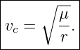
Thus the circular speed is
This formula is only a circular-orbit special case. The general equation of motion remains
At 400 km altitude around Earth,
Thus a spacecraft can experience roughly 8.69 m/s2 of inward acceleration while maintaining
altitude because its transverse velocity continually carries it around Earth as gravity bends its
path.
13 Radial motion as another special case
If the velocity is exactly radial and no transverse component exists, the motion remains on a radial
line. Let r now denote a signed radial coordinate along that line outside the source. The equation
reduces to
This is a one-dimensional nonlinear free-fall equation. It is not the general orbital problem because
ordinary orbits possess transverse motion.
The contrast is important:
whereas in a circular orbit
General Keplerian motion lies between these special cases.
14 Two finite masses: inertial equations
The fixed-source equation is extremely useful when one body overwhelmingly dominates the
mass. However, Newtonian gravity acts on both bodies. Let two masses have inertial
positions
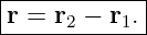
Define the relative vector from body 1 to body 2:
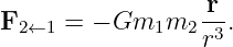
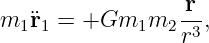
The force on body 2 due to body 1 is
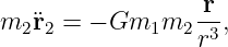
Therefore
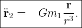
and cancellation of m2 gives
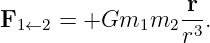
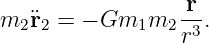
By Newton’s third law, the force on body 1 is opposite:
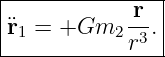
Hence
Equal and opposite forces therefore do not imply equal and opposite accelerations unless the
masses themselves are equal.
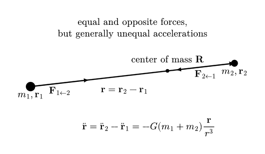
Figure. Both bodies accelerate. Subtracting their inertial accelerations produces a single
relative-motion equation with the combined mass m1 + m2.
15 Deriving the exact relative equation of motion
Differentiate the relative position twice:
Substitute the two body accelerations:
| r | = −Gm1 − Gm2 − Gm2 | (83)
|
| = −G(m1 + m2) . . | (84) |
Therefore
Define the two-body gravitational parameter
Then the exact relative equation becomes
This has exactly the same mathematical form as the fixed-central-mass equation.
The distinction is hidden in the definition of μ:
for the test-particle approximation, but
for exact Newtonian relative two-body motion.
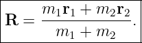
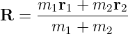
16 The center of mass moves uniformly
Define the center-of-mass coordinate
Differentiate twice:
Using Newton’s equations,
and
The internal forces cancel:
Therefore
So the center of mass moves at constant velocity when no external force acts on the
pair.
CM08 will return to this reduction in greater depth and introduce the reduced mass. For CM03,
the essential point is that the internal two-body dynamics can already be represented by one
relative vector obeying the familiar central-force equation.
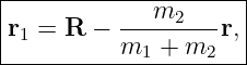
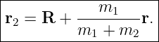
17 Recovering the individual positions from R and r
The definitions
and
can be solved for the two body positions:
Thus the relative orbit does not imply that either body literally sits at the origin. Both bodies
orbit their common center of mass unless one mass is negligible compared with the
other.
This point becomes especially important in binary-star and exoplanet applications, where the
reflex motion of the more massive body is directly observable.
18 The test-particle limit
Suppose
Then
so
The center of mass also lies very close to m1. In that limit, treating the massive body as fixed at
the origin becomes an excellent approximation.
For a planet orbiting the Sun, or a spacecraft orbiting Earth, this approximation is often extremely
accurate. For comparable-mass binary stars, it is not.
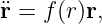
19 First structural consequence: gravity is a central acceleration
The orbital equation has the form
with
Therefore
This fact will be central in CM04. It implies zero torque about the force center and leads directly
to conservation of specific orbital angular momentum:
CM03 does not yet need that conservation law to establish the dynamics, but the structure of
Newton’s orbital equation already contains it.
20 What information is needed to predict an orbit?
For a known gravitational parameter μ, the Newtonian point-mass orbit is determined by six scalar
initial conditions:
and
Equivalently, we specify
Those six numbers are the Cartesian state of the body at an epoch.
Later, CM15 will show that the same ideal two-body orbit can be described geometrically by six
classical orbital elements. The state-vector description and orbital-element description are two
different coordinate descriptions of the same physical trajectory.
21 Astrophysical interpretation
The equation
is not merely a spacecraft equation. It also describes the idealized relative motion of
- two stars in a binary system,
- a star and an exoplanet,
- a planet and a moon,
- a comet and the Sun,
- or a star orbiting a compact central mass when other perturbations are negligible.
The same equation therefore underlies both celestial mechanics and much of observational
astrophysics. Once an orbit can be measured, its geometry and timing can be used to infer
otherwise inaccessible masses.
For example, in an exact Newtonian binary, the relative equation depends on
That is why measured binary orbits can reveal the total system mass. Later astrophysical
application lessons will develop this connection quantitatively.
22 Where the ideal equation stops being sufficient
The equation
assumes an isolated Newtonian two-body system with spherical or point-like masses. Real systems
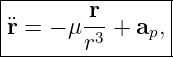
may require additional accelerations:
where ap represents perturbations such as
- gravity from additional bodies,
- nonspherical gravity fields,
- atmospheric drag,
- radiation pressure,
- tidal interactions,
- or relativistic corrections.
The ideal equation is nevertheless the correct starting point because perturbation theory is built by
understanding this solvable core first.
23 Common mistakes
- Writing r = −μ∕r2 without a direction. The left-hand side is a vector, so the right-hand
side must also be a vector.
- Confusing −μr∕r3 with an inverse-cube force. Its magnitude is still μ∕r2 because
|r| = r.
- Forgetting that the position vector must be measured from the chosen force center in
the fixed-central-body approximation.
- Treating velocity as if it always points toward the gravitating body. Gravity constrains
acceleration, not velocity direction.
- Assuming low Earth orbit has negligible gravity. Orbital free fall occurs precisely
because gravity remains strong.
- Using μ = Gm1 for a comparable-mass binary. Exact relative motion uses μ =
G(m1 + m2).
- Assuming equal and opposite gravitational forces produce equal accelerations.
Accelerations differ when masses differ.
- Thinking the differential equation alone selects one orbit. Initial position and velocity
are also required.
- Confusing a state vector (r,v) with orbital elements. They are different representations
of the same ideal orbit.
24 What CM03 adds to the series
CM01 supplied the force law
CM02 supplied the potential description
CM03 now converts those descriptions into dynamics:
For a fixed dominant source,
while exact two-body relative motion uses
Together with
this defines the Newtonian orbital initial-value problem.
The next lessons can now ask what deeper structure is hidden inside this differential equation. The
first answers are conservation of angular momentum and conservation of orbital energy, which will
eventually lead to the conic-section orbit equation.
References
[1] J. M. A. Danby, Fundamentals of Celestial Mechanics, 2nd ed., Willmann-Bell, 1988.
[2] Roger R. Bate, Donald D. Mueller, and Jerry E. White, Fundamentals of
Astrodynamics, Dover Publications, 1971.
[3] John R. Taylor, Classical Mechanics, University Science Books, 2005.
[4] Herbert Goldstein, Charles P. Poole, and John L. Safko, Classical Mechanics, 3rd ed.,
Addison-Wesley, 2001.
[5] Bradley W. Carroll and Dale A. Ostlie, An Introduction to Modern Astrophysics, 2nd
ed., Pearson Addison-Wesley, 2007.












![m3-
[μ ] = [GM ] = s2 .](https://images.physicslibrary.org/cache/objects/1256/make4ht/CelestialMechanicsNewtonsEquationForOrbitalMotion33x.png)

![[ r ] m3 1 m
μ -3 = -2---2 = 2-,
r s m s](https://images.physicslibrary.org/cache/objects/1256/make4ht/CelestialMechanicsNewtonsEquationForOrbitalMotion36x.png)






![[r ]
x = .
v](https://images.physicslibrary.org/cache/objects/1256/make4ht/CelestialMechanicsNewtonsEquationForOrbitalMotion48x.png)
![|----[--------]--|
| v |
|˙x = .|
| − μr ∕r3 |
-----------------](https://images.physicslibrary.org/cache/objects/1256/make4ht/CelestialMechanicsNewtonsEquationForOrbitalMotion49x.png)