Helmholtz Equation, Boundary-Value Problems, and Eigenfunction Expansions
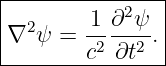
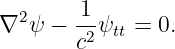
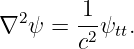
The time-dependent scalar wave equation is
If the motion is harmonic in time, the time dependence can be separated from the spatial
dependence.
Write
Then
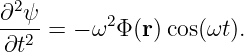
Substitution into the wave equation gives
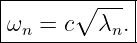
Define
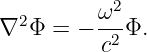
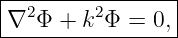
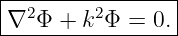
The spatial field therefore satisfies
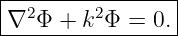
This is the Helmholtz equation.
The central idea of this article is that the differential equation alone is not enough. The
allowed solutions are determined by the differential equation together with the boundary
conditions.
The combination is a boundary value problem.
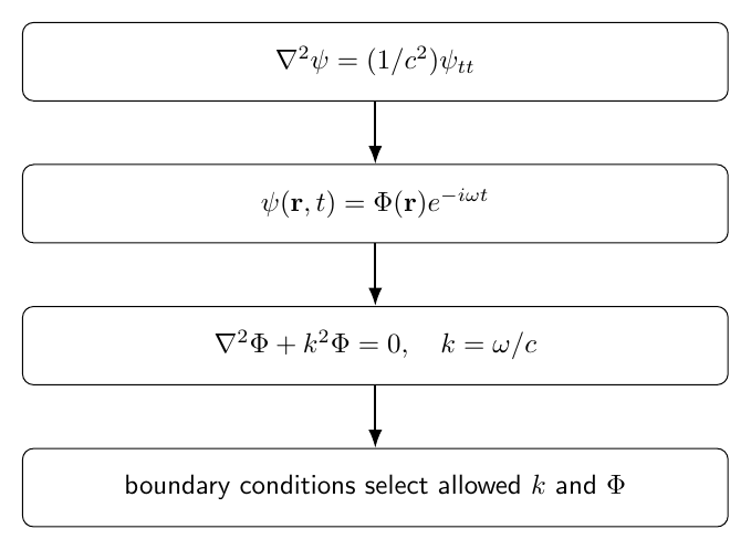
Figure 1. Harmonic time dependence converts the time-dependent wave equation into the spatial
Helmholtz equation. The boundary conditions then select the allowed spatial eigenfunctions and
eigenvalues.
1 From the wave equation to the Helmholtz equation
Start from
Use a complex harmonic representation,
The second time derivative produces
Thus the complex spatial amplitude satisfies
where
The physical field is the real part of the complex representation.
2 Why the Helmholtz equation matters
The Helmholtz equation appears whenever a linear wave system is examined at one angular
frequency.
Examples include:
- vibrating strings,
- vibrating membranes,
- acoustic cavities,
- electromagnetic cavities,
- scalar diffraction models,
- quantum stationary-wave analogues.
The geometry enters through the Laplacian and the boundary conditions.
The allowed values of
become discrete when the domain is bounded and the boundary conditions confine the
field.
3 Boundary value problem
A boundary value problem consists of:
- a differential equation inside a domain,
- boundary conditions specified on the boundary of that domain.
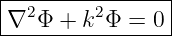
For the Helmholtz equation:
inside a region
the boundary is denoted
Different physical boundaries correspond to different mathematical conditions.
4 Dirichlet boundary condition
A Dirichlet condition specifies the value of the field on the boundary:
The homogeneous Dirichlet condition is
Examples include:
- a string fixed at an endpoint,
- a membrane fixed at its rim,
- a scalar field constrained to vanish on a wall.
M06-17 and M06-18 both used homogeneous Dirichlet conditions.
5 Neumann boundary condition
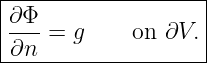
A Neumann condition specifies the Normal derivative:
Here
means derivative in the outward normal direction.
The homogeneous Neumann condition is
Depending on the physical system, this can represent a free boundary, a rigid acoustic wall, or a
no-flux condition.
6 Mixed and Robin boundary conditions
Different parts of the boundary may obey different conditions.
For example:
on one part and
on another.
This is a mixed boundary value problem.
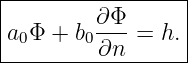
A Robin condition combines field value and normal derivative:
Robin conditions often model finite boundary compliance or impedance-like effects.
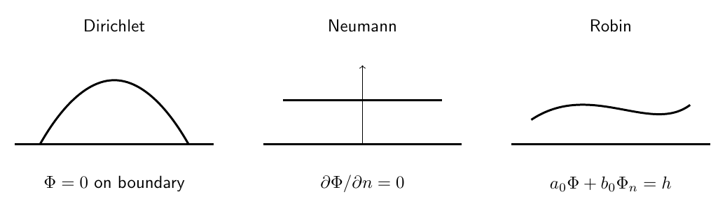
Figure 2. Dirichlet conditions specify the field value, Neumann conditions specify its normal
derivative, and Robin conditions impose a linear combination of both.
7 The Laplacian eigenvalue problem
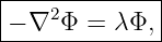
For homogeneous boundary conditions, the Helmholtz equation can be written
where
This is an eigenvalue problem.
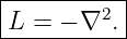
The operator is
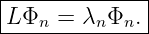
The eigenvalue equation is
The boundary conditions determine which eigenfunctions
and eigenvalues
are allowed.
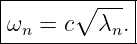
For wave problems,
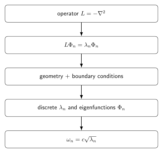
Figure 3. The spatial wave problem is an eigenvalue problem for the negative Laplacian.
Geometry and boundary conditions select a discrete set of eigenfunctions and eigenvalues.
8 One-dimensional fixed interval
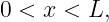
Consider
with
The Helmholtz equation is
Its general solution is
The condition at
gives
The condition at
gives
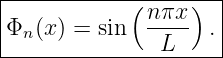
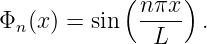
Thus
and
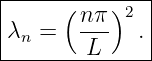
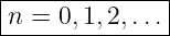
The eigenvalues are
9 One-dimensional Neumann interval
Now impose
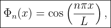
The allowed functions become
with
The
mode is a constant function.
Its eigenvalue is
This zero mode is allowed by Neumann conditions but not by homogeneous Dirichlet
conditions.
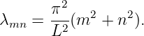
10 Rectangular domain
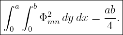
For a rectangle
with
on all four edges, separation gives
and
Thus
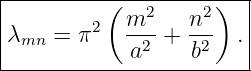
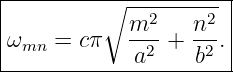
These are exactly the membrane modes derived in M06-17.
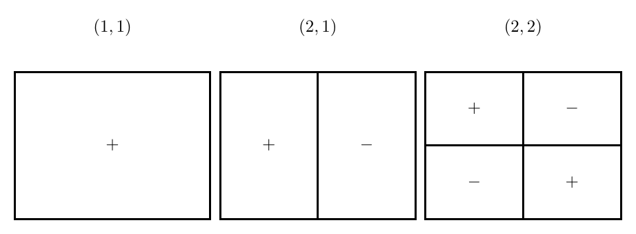
Figure 4. Several rectangular Dirichlet eigenfunctions. The spatial patterns differ, but each
satisfies the same eigenvalue equation with a different allowed value of λ.
11 Circular domain
For a circular domain of radius
with
the separated radial equation becomes Bessel’s equation.
Regularity at the center gives radial factors
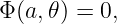
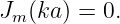
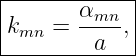
The fixed boundary requires
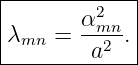
Therefore
and
These are the circular-membrane eigenvalues from M06-18.
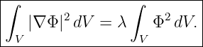
12 Green’s first identity
Orthogonality of Laplacian eigenfunctions can be derived from Green’s first identity:
Interchanging
and
and subtracting gives Green’s second identity:
∫
V  dV = ∫
∂V 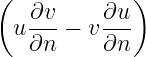 dS. | | (61) |
For homogeneous Dirichlet or homogeneous Neumann boundary conditions, the surface term
vanishes for pairs of eigenfunctions.
13 Orthogonality of distinct eigenfunctions
Let
and
Use Green’s second identity with
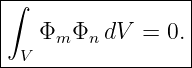
If the boundary term vanishes,
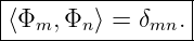
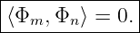
Therefore
If
then
Distinct eigenvalues therefore correspond to orthogonal eigenfunctions.
14 Self-adjointness
An operator
is self-adjoint under an inner product if
for functions satisfying the relevant boundary conditions.
For the Laplacian problem,
Green’s identity shows that the difference between the two inner products becomes a boundary
term.
Homogeneous Dirichlet, homogeneous Neumann, and many suitable Robin conditions make that
term vanish.
This is the structural reason the eigenvalues are real and the eigenfunctions can be chosen
orthogonal.
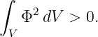
15 Positivity of Dirichlet eigenvalues
For a homogeneous Dirichlet eigenfunction,
Multiply by
and integrate:
Using Green’s first identity and the zero boundary value,
Both integrals are nonnegative.
For a nonzero Dirichlet eigenfunction,
Thus
16 Neumann zero mode
For homogeneous Neumann conditions, a constant function satisfies
and
Therefore
is allowed.
This is why Neumann spectra commonly contain a zero mode.
17 Degeneracy
Two linearly independent eigenfunctions can share the same eigenvalue.
This is degeneracy.
For a square membrane,
Thus
Any linear combination
is also an eigenfunction with that same eigenvalue.
Orthogonality of distinct eigenvalues is automatic.
Within a degenerate eigenspace, one chooses an orthogonal basis.
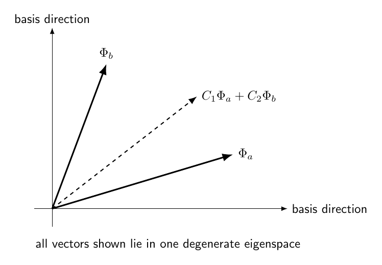
Figure 6. Degenerate eigenfunctions share one eigenvalue. Any linear combination stays within
the same eigenspace, so an orthogonal basis may be chosen for convenience.
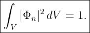
18 Eigenfunction normalization
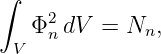
An eigenfunction may be multiplied by any nonzero constant without changing its eigenvalue.
It is often convenient to normalize:
Then
For non-unit normalization,
where
is the normalization constant.
19 Eigenfunction expansion
For many regular bounded domains and standard self-adjoint boundary conditions, the
eigenfunctions form a complete basis for functions satisfying the appropriate conditions.
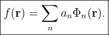
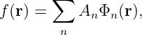
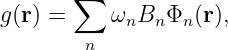
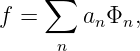
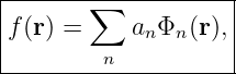
Then a field
can be expanded as
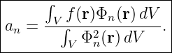
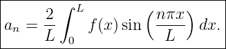
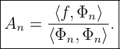
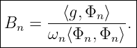
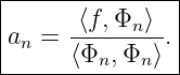
For an orthogonal but not necessarily normalized basis,
This is the multidimensional generalization of Fourier coefficients.
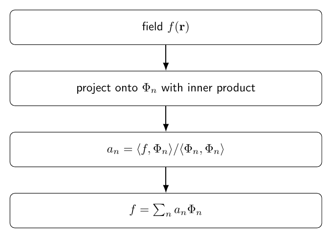
Figure 5. An arbitrary field is projected onto orthogonal eigenfunctions. Each projection
coefficient measures how much of one spatial mode is present in the field.
20 Example 1: sine expansion on a fixed interval
On
with homogeneous Dirichlet conditions,
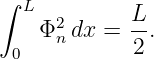
The normalization is
Therefore
This is the ordinary Fourier sine series.
21 Example 2: one exact eigenfunction
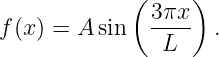
Suppose
Orthogonality gives
and
A field already equal to one eigenfunction has exactly one nonzero modal coefficient.
22 Example 3: rectangular eigenfunction expansion
For the rectangle of M06-17,
The normalization is
Thus
This is the two-dimensional Fourier sine expansion.
23 Example 4: circular eigenfunction expansion
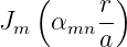
For the circular membrane, the basis functions contain
times sine or cosine angular factors.
The area element is
Thus the radial inner product carries the Weight
For fixed
the radial orthogonality relation is
for
This is the Fourier-Bessel analogue of sine-series orthogonality.
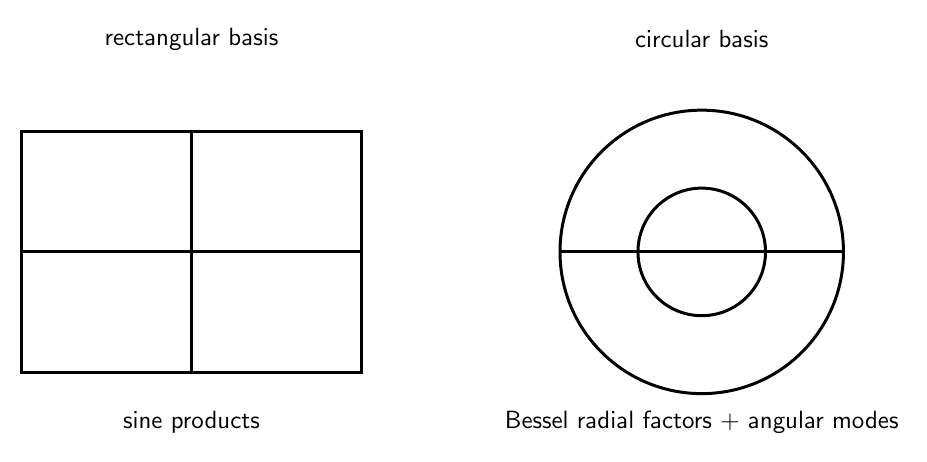
Figure 7. The circular Helmholtz eigenproblem uses the same eigenfunction-expansion logic as a
rectangle, but the radial basis is formed by Bessel functions and the radial inner product carries
the polar weight r.
24 Recovering time-dependent wave motion
Once the spatial eigenfunctions are known, the full wave field is expanded as
Substitute into the wave equation:
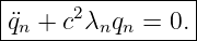
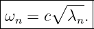
Using
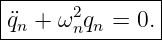
orthogonality separates the modal equations:
Thus
Every spatial eigenfunction becomes one independent normal coordinate.
25 Initial displacement and initial velocity
Let
and
Write
Then
so
Also
so
26 Modal reconstruction
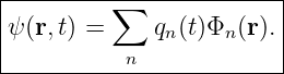
The complete solution is
| ψ(r,t) | = ∑
nΦn(r) . | (119) |
The problem has therefore been decomposed into:
- a spatial eigenvalue problem,
- projection of the initial data,
- independent harmonic evolution of each mode.
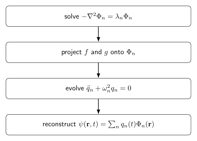
Figure 8. The full solution is reconstructed by evolving each eigenfunction coefficient as an
independent harmonic oscillator and summing the modal contributions.
27 Boundary conditions change the spectrum
The differential operator may stay the same while the spectrum changes because the boundary
conditions change.
For example, on
Dirichlet conditions give
with
Neumann conditions give
with
Thus the boundary is part of the physics, not an afterthought.
28 Boundary geometry changes the basis
Rectangular geometry produces products of sine and cosine functions.
Circular geometry produces Bessel functions and angular trigonometric factors.
Spherical geometry produces spherical Bessel functions and spherical harmonics.
The underlying operator may still be the Laplacian.
The geometry determines the natural coordinate system and the corresponding eigenfunctions.
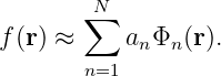
29 Completeness and approximation
In practical calculations, an infinite eigenfunction expansion is truncated:
As more modes are included, the approximation generally improves for sufficiently regular
functions.
Sharp spatial features require higher spatial-frequency modes.
This is the multidimensional analogue of Fourier-series convergence.
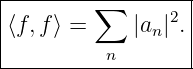
30 Parseval-type relation
For an orthonormal eigenbasis,
the squared norm is
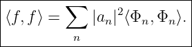
For non-unit normalization,
This is the eigenfunction version of Parseval’s relation.
31 Why eigenfunction expansions are powerful
A partial differential equation can couple infinitely many spatial points.
The eigenfunction basis reorganizes the same problem into independent modal coordinates.
For the homogeneous wave equation,
For forced wave equations, each mode becomes a driven oscillator.
That is the next step developed in M06-20.
32 Common mistakes
- Treating the Helmholtz equation as time dependent.
- Forgetting that k = ω∕c.
- Solving the differential equation without imposing boundary conditions.
- Assuming the same boundary conditions produce the same spectrum in every geometry.
- Confusing Dirichlet field values with Neumann normal derivatives.
- Forgetting the outward normal derivative in a Neumann condition.
- Assuming homogeneous Dirichlet and homogeneous Neumann spectra have the same
lowest mode.
- Forgetting the Neumann zero mode.
- Writing the eigenvalue equation with inconsistent signs.
- Assuming any two eigenfunctions are orthogonal even when they belong to a degenerate
eigenvalue and have not been orthogonalized.
- Forgetting that boundary terms determine whether the Laplacian is self-adjoint.
- Ignoring the geometry-dependent integration measure in the inner product.
- Forgetting the radial weight r in polar coordinates.
- Using expansion coefficients without dividing by the eigenfunction norm.
- Treating completeness as meaning a finite number of modes reproduces every function
exactly.
33 Practice exercises
- Derive the Helmholtz equation from the wave equation using harmonic time
dependence.
- Show that k = ω∕c has units of inverse length.
- State homogeneous Dirichlet, Neumann, and Robin boundary conditions.
- Solve the one-dimensional Dirichlet Helmholtz problem on 0 < x < L.
- Solve the one-dimensional Neumann Helmholtz problem and identify the zero mode.
- Re-derive the rectangular eigenvalues of M06-17 from the Laplacian eigenvalue
problem.
- Re-derive the circular eigenvalues of M06-18 from Jm(ka) = 0.
- Use Green’s second identity to prove orthogonality for distinct eigenvalues.
- Show that homogeneous Dirichlet Laplacian eigenvalues are positive.
- Explain why a homogeneous Neumann problem may contain λ = 0.
- Normalize the one-dimensional Dirichlet eigenfunctions.
- Derive the general projection coefficient for a non-unit orthogonal eigenbasis.
- Derive the modal equations for the full time-dependent wave field.
- Derive the initial-displacement and initial-velocity coefficients.
- Explain why a change in boundary conditions changes the eigenvalue spectrum even if
the differential operator is unchanged.
34 Summary
Harmonic time dependence converts the wave equation into
Equivalently,
The boundary conditions select the allowed eigenfunctions and eigenvalues.
For wave motion,
For distinct eigenvalues under suitable self-adjoint boundary conditions,
A general field can then be expanded as
with
The time-dependent wave field is reconstructed from independent modal oscillators:
The Helmholtz eigenvalue problem therefore supplies the spatial foundation for normal modes,
Resonances, cavity waves, and later forced-wave calculations.
References
References
[1] PhysicsLibrary, M06-18, Circular Membranes, Bessel Functions, and Radial-Angular
Modes.
[2] PhysicsLibrary, M06-17, Separation of Variables, Membranes, and Two-Dimensional
Normal Modes.
[3] PhysicsLibrary, M06-16, Wave Equations in Two and Three Dimensions and
Spherical Waves.
[4] G. B. Arfken, H. J. Weber, and F. E. Harris, Mathematical Methods for Physicists,
7th ed., Academic Press, 2013.
[5] P. M. Morse and H. Feshbach, Methods of Theoretical Physics, McGraw-Hill, 1953.