ED05: Delta Functions, Singular Sources, and Distributions
In ED04, Gauss’ theorem converted the divergence of an Electric Field into a flux through a closed
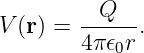
surface. Yet the field of an ideal point charge seems to pose a paradox. For a nonzero distance r
from a charge Q, the Coulomb field is
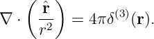
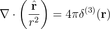
At every such point its ordinary divergence vanishes:
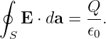
Nevertheless, the outward flux through any sphere containing the charge is
Where does the nonzero divergence reside? The answer is an idealized source concentrated
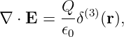
at one point, described by the Dirac delta distribution. The correct global statement
is
This equality is understood in the sense of distributions, not as an ordinary equation evaluated at
r = 0.
We will construct the delta from smooth, finite-width sources; derive its integral properties; extend
it to points, lines, and surfaces; and use it to express charge conservation, electrostatic
Green functions, and a singular current source in Ampere’s law. The theme is simple: a
source can have finite total strength even when its mathematical support shrinks to zero
size.
1 Start with a finite, measurable charge cloud
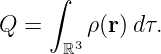
A physical charge distribution has a density ρ(r) and a total charge
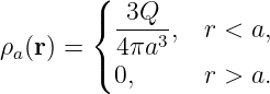
Consider a family of spherical charge clouds, each carrying the same Q, but each having a smaller
radius a:
The density increases as the radius decreases. The total charge does not:
| ∫
ρa dτ | =  ∫
0a4πr2 dr | (7)
|
| =   = Q. | (8) |
As a → 0, the distribution becomes sharply concentrated. Its pointwise limit is zero for every fixed
r≠0, but the integral stays Q. An ordinary function taking value zero at all nonzero points cannot
describe that limit while retaining total charge. The Dirac delta captures exactly the missing
information.
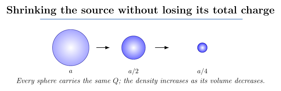
Figure 1. A sequence of uniformly charged balls of decreasing radius, each containing the same
charge Q. Their density increases as a−3, while the integrated charge remains fixed.
2 Constructing the one-dimensional Dirac delta
Before using a three-dimensional point charge, study one coordinate x. A particularly convenient
narrow function is the normalized Gaussian
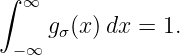
Its integral is one:
This follows by substituting u = x∕σ and using the standard Gaussian integral. Its width is
controlled by σ; its peak height increases as 1∕σ.
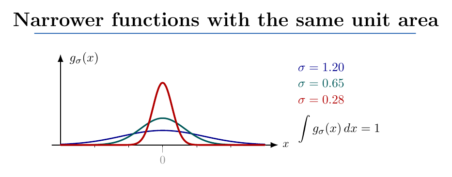
Figure 2. Narrow normalized Gaussians. Every curve has area one, despite differing widths and
peak heights. The delta distribution is obtained from their limiting action on smooth test
functions, not as a finite-height ordinary curve.
Let f be a smooth function that varies little over the narrow peak. Substituting x = σu
gives
| ∫
−∞∞f(x)g
σ(x) dx | =  ∫
−∞∞f(σu)e−u2∕2 du. | (11) |
When σ → 0, the factor f(σu) approaches f(0). Under ordinary smoothness and integrability
assumptions allowing the limit to pass through the integral, we obtain
| lim σ→0 ∫
−∞∞f(x)g
σ(x) dx | = f(0) ∫
−∞∞e−u2∕2 du | (12)
|
| = f(0). | (13) |
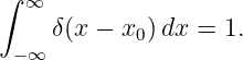
This motivates the defining sifting property
More precisely, δ is a distribution: it is defined by how it acts under integration against a
sufficiently smooth, localized test function. The symbol δ(0) is not an ordinary finite number. A
useful shorthand is that δ(x) = 0 for x≠0 and has unit integral, but the sifting rule is the actual
mathematical definition.
3 Delta normalization, translation, and units
Applying the sifting identity to a test function equal to one near the origin gives
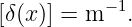
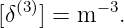
If x has units of length, then dx has units of meters and the one-dimensional delta must have units
of inverse length:
The shifted delta δ(x − x0) is supported at x = x0. Translation changes the location of the source
but not its total strength.
4 Scaling and changing variables
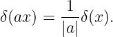
Take a nonzero constant a. For any smooth test function, substitute u = ax (accounting for the
orientation of the integration limits when a < 0):
| ∫
−∞∞f(x)δ(ax) dx | =  ∫
−∞∞f(u∕a)δ(u) du | (17)
|
| =  . | (18) |
Therefore, as distributions,
The absolute value is essential. A change of coordinate orientation cannot turn a positive sampling
Weight into a negative one.
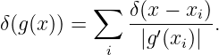
A broader rule is useful. Suppose g(x) has isolated, simple zeros xi, meaning g(xi) = 0 and
g′(xi)≠0. In a small neighborhood of each root,
Applying Equation (19) near each root gives
This rule is valid only when the roots are simple; at a repeated zero, this formula is not directly
applicable.
Example: a shifted quadratic
For g(x) = x2 − a2 with a > 0, the roots are ±a, and g′(±a) = ±2a. Thus
Consequently,
where the integral is over the real line.
5 Why differentiation of delta functions is possible
An ordinary derivative does not exist at a delta’s support. A distributional derivative is defined by
moving the derivative onto the test function using integration by parts:
The minus sign is not arbitrary. It comes from the integration-by-parts formula
with vanishing boundary terms for compactly supported test functions. Taking T = δ(x − x0)
produces Equation (24).
This is a general strategy: fields that cannot be differentiated in the ordinary sense may still have
well-defined derivatives after integration against smooth probes.
6 The three-dimensional delta
In three-dimensional Cartesian coordinates, define
For a smooth localized test function f,
The units now are
A point charge Q at r0 is therefore represented by
Integrating over any volume containing r0 yields Q, while a region not containing r0 yields zero.
This is exactly the behavior required of a point charge.
7 Ideal point, line, and sheet charge sources
Ideal sources need not be concentrated in all three dimensions. The appropriate number of delta
factors is determined by how many transverse coordinates collapse to zero.
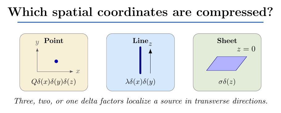
Figure 3. Point, line, and sheet sources as increasingly extended idealizations. A point is localized
in three coordinates, a line in two transverse coordinates, and a sheet in one normal coordinate.
Point charge
A charge Q at the origin has
The coefficient Q has SI units of coulombs.
Infinite line charge
For a line charge on the z axis with linear charge density λ,
Consider a cylinder of length L whose cross-section contains the axis. The charge is
| QL | = ∫
0Ldz ∫
∫
λδ(x)δ(y) dxdy | (32)
|
| = λL. | (33) |
The coefficient has units [λ] = C∕m, while the two delta factors supply m−2, yielding the correct
volume-density units C∕m3.
Infinite plane charge
For a uniform charged plane in z = 0 with surface charge density σ,
Integrating through a slab with footprint area A gives Q = σA. Here [σ] = C∕m2 and
[δ(z)] = m−1.
For a smooth curved surface described locally by a signed-distance coordinate n, a surface charge
can similarly be written ρ = σδ(n) with the geometry encoded in the volume measure. For a
general level-set function g(r), the corresponding form is ρ = σ|∇g|δ(g), provided ∇g≠0 on the
surface and σ is defined there.
8 Coordinate forms of concentrated sources
The Cartesian product form is often the safest starting point. In cylindrical coordinates
(s,ϕ,z),
The transverse delta supported at the z axis is commonly written
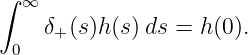
Here δ+(s) is the one-sided delta at the endpoint s = 0, defined so that
The quotient in Equation (36) is a distribution defined with the cylindrical measure. To verify its
normalization for a continuous function f(x,y), integrate:
∫
02π∫
0∞f(s,ϕ) sdsdϕ | =  ∫
02πf(0,ϕ) dϕ | (38)
|
| = f(0, 0). | (39) |
At the axis the different azimuth values identify the same physical point, so f(0,ϕ) is independent
of ϕ.
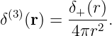
Likewise, in spherical coordinates,
and the three-dimensional delta at the origin may be represented as
Indeed, applying the right-hand side to a smooth f and integrating with the spherical volume
element gives
| ∫
0∞∫
0π∫
02πf(r,𝜃,ϕ) r2 sin 𝜃 dϕd𝜃 dr | (42)
|
| =  ∫
0π∫
02πf(0,𝜃,ϕ) sin 𝜃 dϕd𝜃 = f(0). | (43) |
These endpoint formulas are useful shorthand, but the Cartesian sifting property should be used
whenever the meaning of a radial delta at r = 0 is unclear. In particular, writing an ordinary
full-line δ(r) without specifying the endpoint convention can introduce a spurious factor of
two.
9 From a small charged sphere to a singular Coulomb field
Return to the uniformly charged ball in Equation (6). By spherical symmetry, its electrostatic field
is radial:
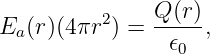
Gauss’s Law on a sphere of radius r < a gives
where Q(r) = Q(r3∕a3) is the charge enclosed. Hence
Outside the sphere,
The field is continuous at r = a, though its radial derivative changes there because the charge
density jumps. For r < a, the ordinary divergence is
| ∇⋅ Ea | =  ∇⋅ (xx + yy + zz) | (48)
|
| =  =  . | (49) |
For r > a, its ordinary divergence is zero. Thus the divergence of the smooth-inside, piecewise field
is exactly the finite source density divided by 𝜖0.
As a → 0, the volume supporting the divergence collapses while its integral stays Q∕𝜖0.
Hence
which, after substituting Equation (1), is Equation (4).
10 A direct proof using a test function
We can establish Equation (4) without choosing a particular approximating charge cloud.
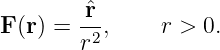
Let
For a compactly supported smooth test function f, distributional divergence is defined
by
The integral converges locally because |F|∼ r−2 and dτ ∼ r2dr dΩ.
Exclude a ball r < 𝜀, apply the divergence theorem on the region outside the ball, and take 𝜀 → 0.
Since ∇⋅ F = 0 for r > 0,
| ∫
r>𝜀F ⋅∇f dτ | = ∮
r=𝜀fF ⋅ (−r) da | (53)
|
| = −∫
4πf(𝜀, Ω) dΩ. | (54) |
The inner boundary Normal for the punctured region is −r. Because f is continuous at the
origin,
Combining with Equation (52),
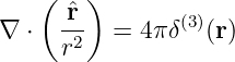
Because this holds for every such test function,
as distributions.
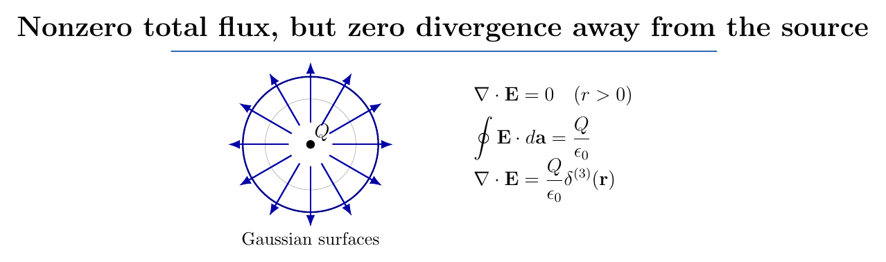
Figure 4. An inverse-square field has zero ordinary divergence at every nonzero radius, yet the
flux through every centered closed sphere is 4π for the normalized field r∕r2. Its distributional
divergence is a delta at the origin.
11 The electrostatic potential and Poisson’s equation
Away from the origin, the Coulomb potential is
The field is
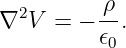
Taking its divergence and using Gauss’s law yields Poisson’s equation,
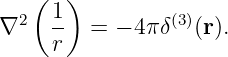
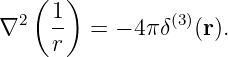
For a point charge, substitute V = Q∕(4π𝜖0r) and ρ = Qδ(3)(r). The result is the fundamental
identity
This is the same physics as the divergence identity, with the minus sign arising from
E = −∇V .
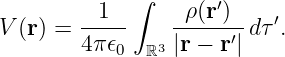
If ρ(r′) is localized and we choose a potential that vanishes sufficiently far away, superposition
gives
Differentiate with ∇r2 and use the shifted version of Equation (61):
Then
| ∇2V (r) | = − ∫
ρ(r′)δ(3)(r − r′) dτ′ | (64)
|
| = − . | (65) |
Thus the Coulomb kernel 1∕(4π|r − r′|) acts as a Green function for −∇2 on unbounded
three-dimensional space. Boundaries can require an additional harmonic solution or a
boundary-adapted Green function; the free-space kernel alone does not automatically satisfy
Conductor boundary conditions.
12 A charged plane as a distributional jump
For a uniform infinite sheet at z = 0, Gauss’s law and reflection symmetry give
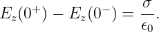
where sgn(z) = +1 for z > 0 and −1 for z < 0. This electric field is constant on either side. It
jumps by
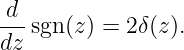
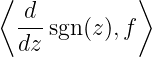
The sign function has distributional derivative
To verify this, write its action on a compactly supported smooth f:
 | = −∫
−∞∞ sgn(z)f′(z) dz | (69)
|
| = −∫
0∞f′(z) dz + ∫
−∞0f′(z) dz | (70)
|
| = 2f(0). | (71) |
Therefore
precisely matching the sheet charge density in Equation (34).
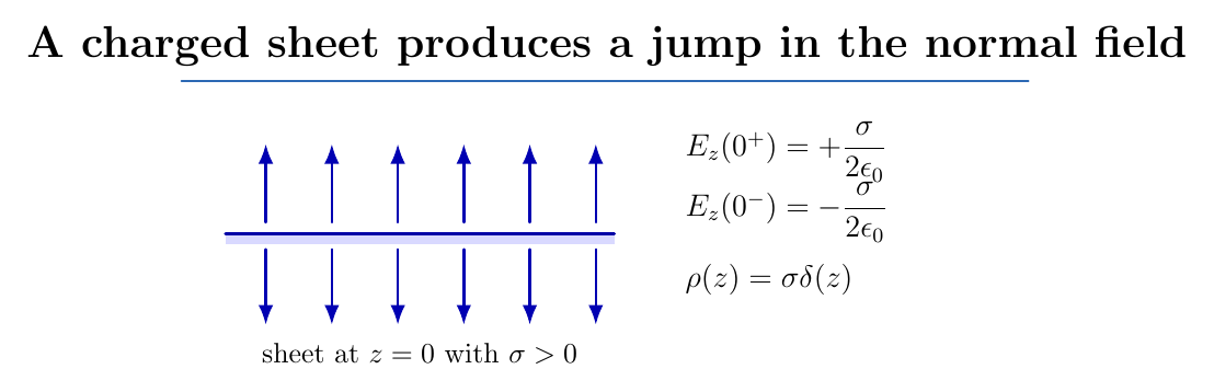
Figure 5. A uniform charged sheet produces an electric field that points in opposite normal
directions on the two sides. The field jump becomes a delta-function divergence localized on the
sheet.
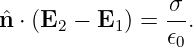
A more general electrostatic boundary result follows from the same pillbox argument:
The normal n points from region 1 to region 2. This relation is not a new charge law: it is Gauss’s
law applied to a singular surface source.
13 An ideal straight wire and singular magnetic curl
Consider an infinitely long wire on the z axis carrying steady current I along +z. The volume
current density is
Ampere’s law gives the familiar azimuthal magnetic field
Outside the axis, cylindrical curl gives
Yet any circular path enclosing the axis has circulation
| ∮
B ⋅ dl | =  (2πs) = μ0I. | (77) |
Stokes’ theorem, interpreted distributionally for the singular field, implies
The curl is zero at each ordinary point with s > 0 but has a concentrated contribution on the wire.
Equation (78) agrees exactly with the magnetostatic Ampere law ∇× B = μ0J.
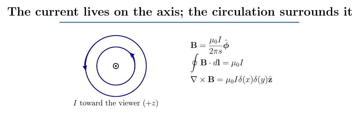
Figure 6. The magnetic field of a line current circulates around the wire. Every loop enclosing the
wire has the same integral μ0I, while loops avoiding the axis bound surfaces on which the
ordinary curl vanishes.
14 A moving point charge and the continuity equation
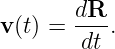
So far the ideal sources were static. Let a point charge q follow a differentiable path R(t) with
velocity
Its charge and current densities are
We can check charge conservation without requiring a nonsingular charge cloud. Differentiate the
shifted delta with respect to time, using the chain rule in the distributional sense:
Because v(t) is independent of the field coordinate r,
Add the two expressions:
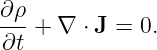
The continuity equation therefore holds even for an ideal point particle: it is an identity about
distributions. A time-dependent ρ and J do not, by themselves, determine instantaneous fields
through the static Coulomb or Biot-Savart formulas. Electromagnetic propagation and retardation
are needed for the time-dependent field problem.
15 A point dipole as a derivative of a delta
A deeper example shows why derivatives of delta distributions are useful. Place a charge +q at
+a∕2 and a charge −q at −a∕2:
For small a, Taylor-expand the shifted deltas as distributions:
| δ(3)(r − a∕2) | = δ(3)(r) − ⋅∇δ(3)(r) +  , | (86)
|
| δ(3)(r + a∕2) | = δ(3)(r) +  ⋅∇δ(3)(r) +  . | (87) |
Subtracting gives
where p = qa is the dipole moment pointing from the negative to the positive charge. In the
ideal-dipole limit, |a|→ 0 and q is scaled so that p stays fixed.
Check this representation by integrating the density against a test potential f:
| ∫
ρ(r)f(r) dτ | = 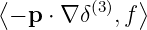 | (89)
|
| = p ⋅∇f(0). | (90) |
The source has no net charge, but it retains first-order information about spatial variation. This
observation connects delta distributions naturally to multipole expansions.
16 Regularity, singularities, and common pitfalls
Several distinctions matter in calculations:
- A field may be smooth away from a source but singular at its support. Differential
identities valid only for r > 0 cannot be extended to r = 0 without a distributional
argument.
- The delta is not an ordinary function with an infinitely tall, infinitesimally narrow
graph. Its action under integration is the defining statement.
- coordinate singularities are not automatically physical sources. The azimuthal basis
degenerates at s = 0 even for perfectly regular Cartesian fields. A genuine distributional
source must be established by flux, circulation, or test-function methods.
- A field discontinuity need not be an infinite field. A finite jump can have a
delta-function derivative, as with a charged sheet.
- The expression δ(r)∕r2 at the radial endpoint requires a convention. Use the one-sided
normalization or return to δ(3)(r).
- Multiplying or otherwise combining arbitrary singular distributions is not
automatically defined. The linear operations used here are well-defined for the displayed
examples.
- Approximating a point source with a finite charge cloud resolves a mathematical
singularity but does not automatically describe atomic-scale or quantum physics.
17 Worked example 1: charge inside a Gaussian volume
A point charge Q = 3.0 nC is located at (a, 0, 0), where a = 0.020 m. Its charge density
is
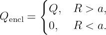
Let a spherical Gaussian volume be centered at the origin with radius R. Integrating the source
over the volume yields
At R = a, a surface passes through the point source and a limiting convention or more detailed
geometry is needed. For R > a, Gauss’s law gives flux
The electric field need not have constant magnitude over the sphere because the source is off
center. Gauss’s law determines the total flux, not the full field geometry.
18 Worked example 2: an infinite charged sheet
Suppose σ = 5.0 nC∕m2 on z = 0. The electric field on either side has magnitude
| E | =  ≈ 282 N∕C. | (94) |
Its jump is approximately 565 N∕C. The charge density is ρ = σδ(z), with the correct units C∕m3.
The distributional divergence produces precisely σδ(z)∕𝜖0, showing that the discontinuous field and
the sheet source satisfy local Gauss’s law.
19 Worked example 3: an infinite wire
For I = 2.0 A, the magnetic field at s = 5.0 cm is
| Bϕ | =  ≈ 8.0 × 10⁻⁶ T. | (95) |
Its circulation around that circle is
consistent with μ0I. The nonzero circulation is accounted for by the delta-supported current and
the distributional curl at the axis.
20 Worked example 4: regularized point charge
A sphere of radius a = 0.010 m carries Q = 1.0 nC uniformly. The volume charge density
is
Inside, the field grows linearly with radius. At r = a,
The total outward flux through any concentric sphere of radius r > a is Q∕𝜖0, independent of a. As
a decreases, the field for any fixed r > 0 remains the same, but the divergence concentrates into a
smaller source region.
21 Practice exercises
- Verify the normalization of the Gaussian family in Equation (9) by the substitution
u = x∕σ.
- Use the scaling rule to simplify δ(3x − 6).
- For a > 0, evaluate ∫
−∞∞x2δ(x2 − a2) dx.
- Determine the SI units of δ(2)(r
⊥) and check the line-charge density units.
- Integrate ρ = σδ(z − z0) through a slab whose thickness includes z0.
- Derive the electric field within a uniformly charged solid ball from Gauss’s law.
- Starting from F = r∕r2, compute the flux through a sphere of arbitrary radius and
explain why ordinary divergence does not describe the origin.
- Show that ∇2(1∕r) = 0 for r > 0, and explain why this does not contradict
Equation (61).
- For a line current along +z, compute ∮
B ⋅ dl on two circles of different radii, both
enclosing the axis.
- Verify the continuity equation for ρ and J of a point charge moving at constant velocity
v.
- Explain why a field with finite one-sided limits but a jump at a sheet can have a
delta-supported divergence.
- Derive the ideal-dipole source −p ⋅∇δ(3) from two separated charges by acting on a
smooth test function.
22 Summary and bridge to ED06
The delta distribution represents a localized source through its integral action. A point charge, line
charge, and sheet charge use three, two, and one transverse delta factors, respectively. Its
derivative is defined by integration by parts. The fundamental electrostatic identities
are
and
An infinite charged plane generates a field jump and delta-supported divergence; a line current
generates nonzero circulation and delta-supported curl. A moving point charge obeys the
continuity equation in the distributional sense.
ED06 returns to curvilinear coordinates, where the metric scale factors and the correct volume
measure allow us to distinguish coordinate artifacts from genuine singular sources. Together,
ED02 through ED06 provide the mathematical vocabulary needed for electrostatics and
magnetostatics.
References
[1] D. J. Griffiths, Introduction to Electrodynamics, 5th ed., Cambridge University Press,
2023.
[2] H. M. Schey, Div, Grad, Curl, and All That, 4th ed., W. W. Norton, 2005.
[3] J. D. Jackson, Classical Electrodynamics, 3rd ed., Wiley, 1999.
[4] F. G. Friedlander and M. Joshi, Introduction to the Theory of Distributions, 2nd ed.,
Cambridge University Press, 1998.