Strapdown Inertial Navigation Examples: Effective Gravity and Navigation Equations
This companion to INS05 turns the gravity models and rotating-Earth equations into explicit
calculations. The central bookkeeping distinction is
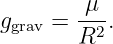
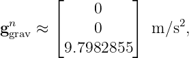
where ggrav is gravitation from Earth’s mass distribution and g is effective gravity for a rotating
Earth-fixed mechanization.
The examples use the WGS-84 constants
and the Somigliana constants
The notation and sign conventions follow INS05 and standard inertial-navigation references
[1, 2, 3, 4].
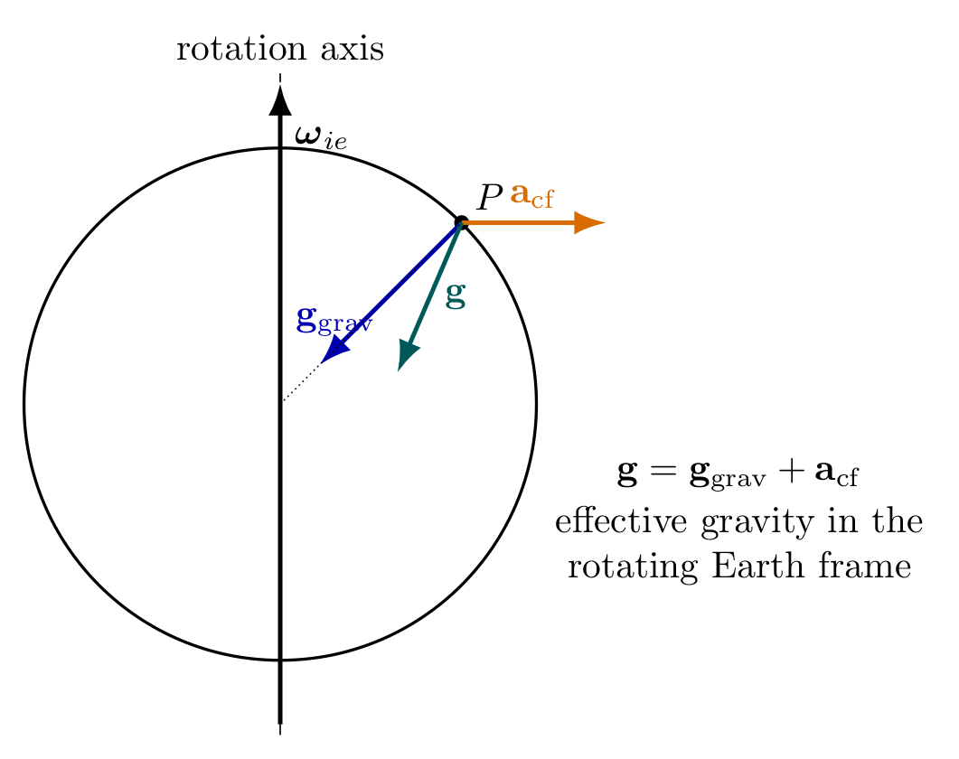
Figure. In the spherical model, gravitation points toward Earth’s center while the
centrifugal acceleration points away from the rotation axis. Their vector sum is the
effective gravity used by the rotating-Earth navigation equation.
1 Exercises
Exercise 1: Point-mass gravitation and effective gravity at the equator
At the WGS-84 semi-major radius R = a, approximate Earth as a spherical point mass.
- Compute the point-mass gravitational acceleration magnitude
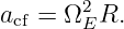
- Compute the equatorial centrifugal acceleration
- Compute the simple spherical effective gravity at the equator.
- Compare it with WGS-84 Normal gravity at the equator and explain why the two are not
expected to be identical.
Exercise 2: Centrifugal acceleration resolved in NED
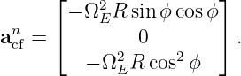
Use a spherical Earth of radius R = a at latitude ϕ = 45∘. For a point fixed to Earth, show that
the centrifugal acceleration resolved in local NED is
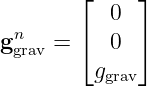
Compute the numerical vector. Then combine it with spherical gravitation
to find the effective gravity vector, its magnitude, and its angular deflection from the local radial
down direction.
Exercise 3: WGS-84 normal gravity from Somigliana’s formula
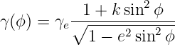
Evaluate
at ϕ = 30∘, 45∘, and 60∘.
- Compute all three values.
- Compute the difference between 60∘ and 30∘.
- Explain why this latitude variation matters to a strapdown INS.
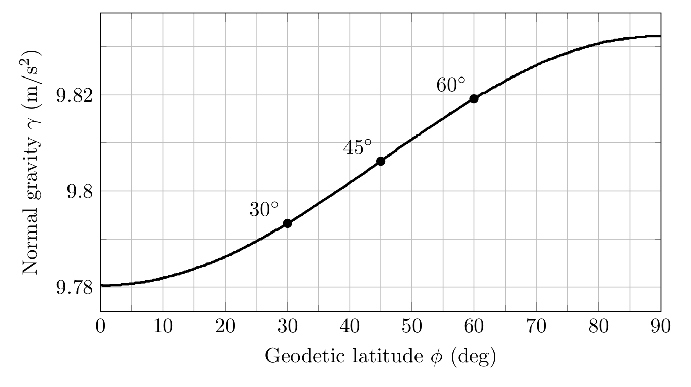
Figure. WGS-84 normal gravity increases with geodetic latitude. The variation is large
compared with inertial-sensor error levels, so using one constant value of g is not a
high-quality navigation model.
Exercise 4: First-order normal-gravity correction with altitude
At latitude 45∘, use the simple first-order height approximation
Find normal gravity at h = 2.00 km and calculate the reduction from the ellipsoid-surface
value.
Exercise 5: Stationary accelerometer sanity check in NED
A level IMU is stationary relative to Earth at latitude 45∘ and height h = 0. Neglect local gravity
anomalies and use WGS-84 normal gravity.
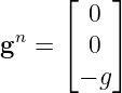
- Write gn in NED.
- Find the ideal accelerometer specific force fn.
- Substitute the values into the local NED velocity equation with vebn = 0 and verify
that the velocity derivative vanishes.
- State the most common sign error this example exposes in navigation code.
Exercise 6: ECEF velocity equation for eastward motion at the equator
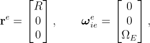
Use the simple spherical Earth model at the equator and longitude zero. Let
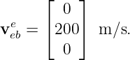
and suppose the vehicle has constant ECEF east velocity
- Compute ggrave.
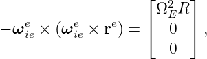
- Compute the explicit centrifugal acceleration.
- Compute effective gravity ge.
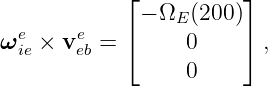
- Compute the Coriolis contribution −2ωiee × v
ebe.
- Find the specific-force vector required for dvebe∕dt = 0 in this idealized example.
Exercise 7: Proving the two ECEF gravity forms are equivalent
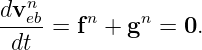
Start with
Use the definition of effective gravity to derive
Then explain precisely why adding another centrifugal term to the second equation would be
incorrect.
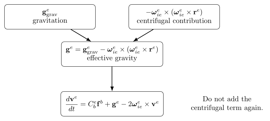
Figure. The explicit-gravitation and effective-gravity ECEF forms are equivalent
descriptions. The centrifugal contribution belongs in exactly one place.
Exercise 8: Full numerical NED velocity update
At
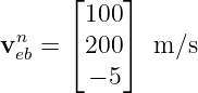
a vehicle has
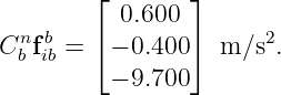
and transformed specific force
Use
and
Compute
Use the first-order altitude correction for γ(45∘, 1000 m).
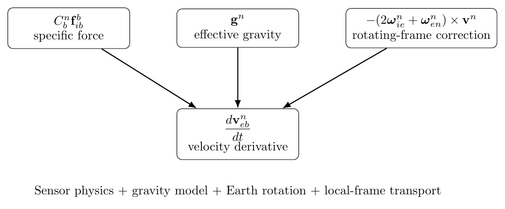
Figure. A local-level velocity update combines transformed specific force, gravity, Earth
rate, transport rate, and the current velocity. Each term has a distinct physical origin.
Exercise 9: What double-counting centrifugal acceleration does
At the equator, suppose a programmer uses WGS-84 effective gravity but also subtracts a separate
centrifugal term of magnitude approximately
Treat the resulting acceleration error as constant for 60 s.
- Find the acceleration error magnitude.
- Find the resulting velocity error after 60 s.
- Find the resulting position error from rest using δr =
 δat2.
δat2.
Exercise 10: Gravity-model error accumulation
A gravity model has a constant vertical error of 50 mGal. Recall that
Assume no aiding and neglect all other errors.
- Convert the gravity error to SI acceleration units.
- Find the vertical velocity error after 300 s.
- Find the corresponding position error from rest.
- Explain why this simple t2 result is only a short-time approximation for a full navigation
system.
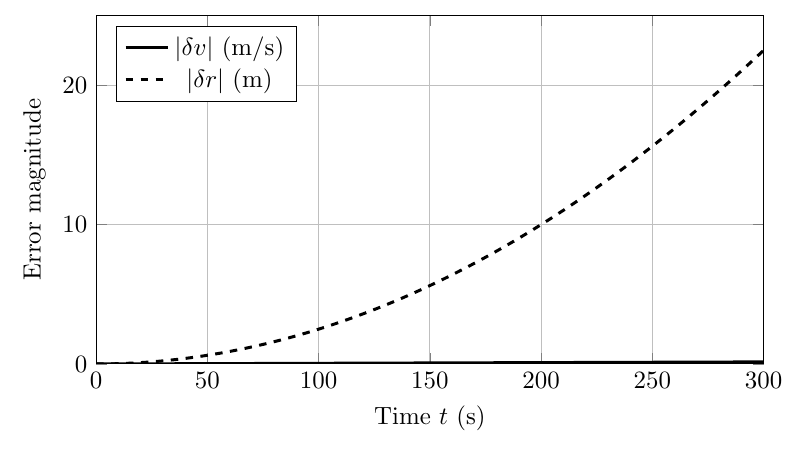
Figure. A constant gravity-model acceleration error integrates once into velocity error and
twice into position error. This is one reason gravity-model fidelity matters even when the
accelerometers themselves are ideal.
2 Worked solutions
Solution 1: Point-mass gravitation and effective gravity at the equator
Using R = a = 6378137 m,
The centrifugal acceleration at the equator is
In this simple spherical model, both vectors are radial and opposite. Therefore
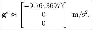
WGS-84 normal gravity at the equator is
The spherical point-mass estimate differs by about
The discrepancy is not a numerical mistake. The point-mass model ignores Earth’s
oblateness and the way the reference ellipsoid and normal gravity field are constructed
together. This comparison is a useful warning: subtracting a centrifugal term from a crude
spherical gravitation model is not the same as evaluating the WGS-84 normal gravity
field.
Solution 2: Centrifugal acceleration resolved in NED
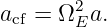
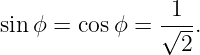
At ϕ = 45∘,
First compute
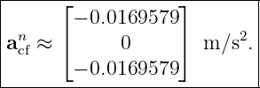
Therefore
and
Hence
Using the point-mass value from Exercise 1,
so
The magnitude is
The angular deflection from radial down is approximately
The horizontal component points toward the equator. In a realistic ellipsoidal model, local geodetic
down is defined so that the normal-gravity field is aligned with the ellipsoid normal, which is why
this spherical result should be treated as a physics illustration rather than a production
local-gravity model.
Solution 3: WGS-84 normal gravity from Somigliana’s formula
Using
Somigliana’s formula gives
and
The difference between 60∘ and 30∘ is
This is roughly 2.6 × 10⁻³g. A strapdown navigator that simply inserts a single constant value of
gravity everywhere creates a deterministic acceleration error that can be much larger than the
errors of a good inertial sensor.
Solution 4: First-order normal-gravity correction with altitude
At 45∘,
At h = 2000 m,
which gives
The reduction is
The approximation captures the dominant inverse-square trend. More accurate normal-gravity
formulas include ellipsoidal height dependence explicitly.
Solution 5: Stationary accelerometer sanity check in NED
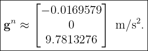
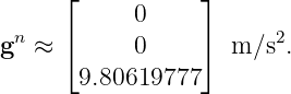
At the surface and 45∘ latitude,
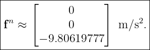
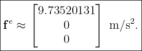
For a stationary supported IMU, INS03 showed that ideal specific force is the negative of effective
gravity:
Because vebn = 0, the Earth-rate and transport-rate cross-product terms vanish. Therefore
This is one of the strongest unit tests for a local-level mechanization. A common mistake is to
use
while simultaneously declaring the navigation frame to be NED. In NED, positive down means the
gravity vector has a positive third component.
Solution 6: ECEF velocity equation for eastward motion at the equator
At longitude zero on the equator,
The explicit centrifugal acceleration is
so
Thus the simple spherical effective gravity is
Now
so
For zero ECEF velocity derivative,
so
The required outward specific force is slightly less than the magnitude of effective gravity because
the Coriolis contribution in this geometry is outward.
Solution 7: Proving the two ECEF gravity forms are equivalent
Define effective gravity by
Substituting this definition into the explicit equation immediately gives
No physics disappeared. The centrifugal contribution was grouped into the definition of
ge.
If a navigation program uses this effective-gravity form and then subtracts another
it counts the rotational contribution twice. This is a bookkeeping error, not a higher-fidelity
model.
Solution 8: Full numerical NED velocity update
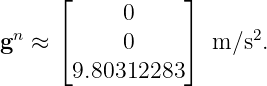
At 45∘ latitude,
and
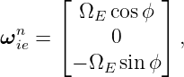
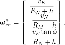
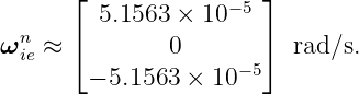
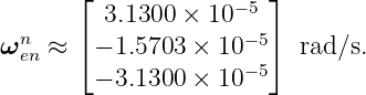
Earth rate resolved in NED is
Using vN = 100 m/s and vE = 200 m/s,
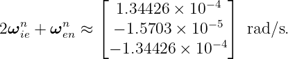
Therefore
The cross product with velocity is
The first-order altitude-corrected gravity is
so
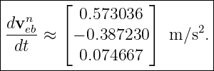
Finally,
which gives
This example shows why the mechanization cannot be interpreted as “rotate accelerometer data
and add g.” The rotating-frame correction is small compared with g, but it is not small compared
with the accelerations a navigation system may be trying to resolve.
Solution 9: What double-counting centrifugal acceleration does
At the equator,
After t = 60 s, the velocity error is approximately
The corresponding position error is
This large error develops in only one minute. The example demonstrates why the definition of the
gravity vector in software must be paired unambiguously with the form of the navigation
equation.
Solution 10: Gravity-model error accumulation
A 50 mGal error is
After 300 s,
The corresponding position error is
The t2 result assumes a constant error direction in a simple Cartesian model. A real local-level INS
couples gravity error, attitude error, Earth curvature, transport rate, and Schuler dynamics. Those
effects will be developed later in the series. The short-time estimate is still valuable because it
reveals the direct double integration mechanism.
3 What these exercises establish
The examples reinforce several implementation rules.
First, gravitation and effective gravity are not interchangeable symbols. The correct choice depends
on the exact navigation equation being implemented.
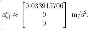
Second, centrifugal acceleration is not a small conceptual detail. At the equator it is
about
which is large compared with precision inertial-sensor errors.
Third, WGS-84 normal gravity already represents the rotating reference ellipsoid. A local-level
mechanization using normal gravity must not add the same centrifugal contribution a second
time.
Fourth, the complete local NED velocity equation
contains terms from sensor physics, gravity modeling, Earth rotation, local-frame motion, and
geometry. Every term has now been derived or calculated explicitly.
Finally, even modest gravity-model errors integrate into navigation errors. Later articles will
show how the full inertial error dynamics modify this simple growth and lead to Schuler
behavior.
References
[1] David H. Titterton and John L. Weston, Strapdown Inertial Navigation Technology,
2nd ed., Institution of Electrical Engineers, 2004.
[2] Paul D. Groves, Principles of GNSS, Inertial, and Multisensor Integrated Navigation
Systems, 2nd ed., Artech House, 2013.
[3] Christopher Jekeli, Inertial Navigation Systems with Geodetic Applications, Walter
de Gruyter, 2001.
[4] National Geospatial-Intelligence Agency, Department of Defense World Geodetic
System 1984: Its Definition and Relationships with Local Geodetic Systems,
NGA.STND.0036, Version 1.0.0, 2014.
[5] Helmut Moritz, “Geodetic Reference System 1980,” Bulletin Geodesique, vol. 54, pp.
395–405, 1980.

![[parent]](https://images.physicslibrary.org/images/uparrow.png)