|
|
|
|||||||
and a wave traveling in the +z direction is written
The exact material relations used repeatedly are
and
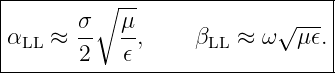
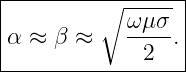
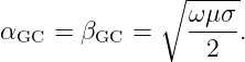
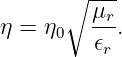
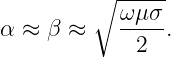
For a good Conductor,
These formulas are consequences of Maxwell’s equations and the constitutive relations, not independent empirical rules [1, 2, 3, 4].
How to use this problem setAttempt all exercises in Part I before consulting Part II. For every problem, first compute or estimate
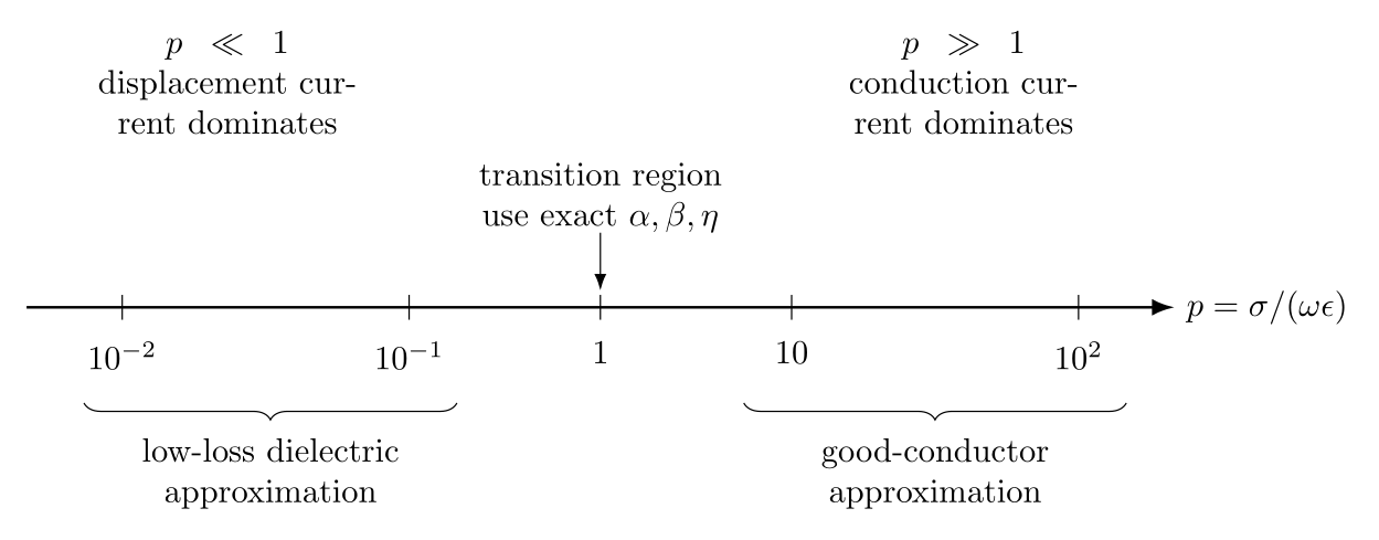
This single dimensionless ratio often tells you whether the lossless, low-loss, exact lossy, or good-conductor formulas are appropriate.
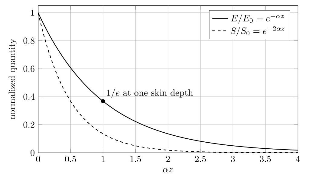
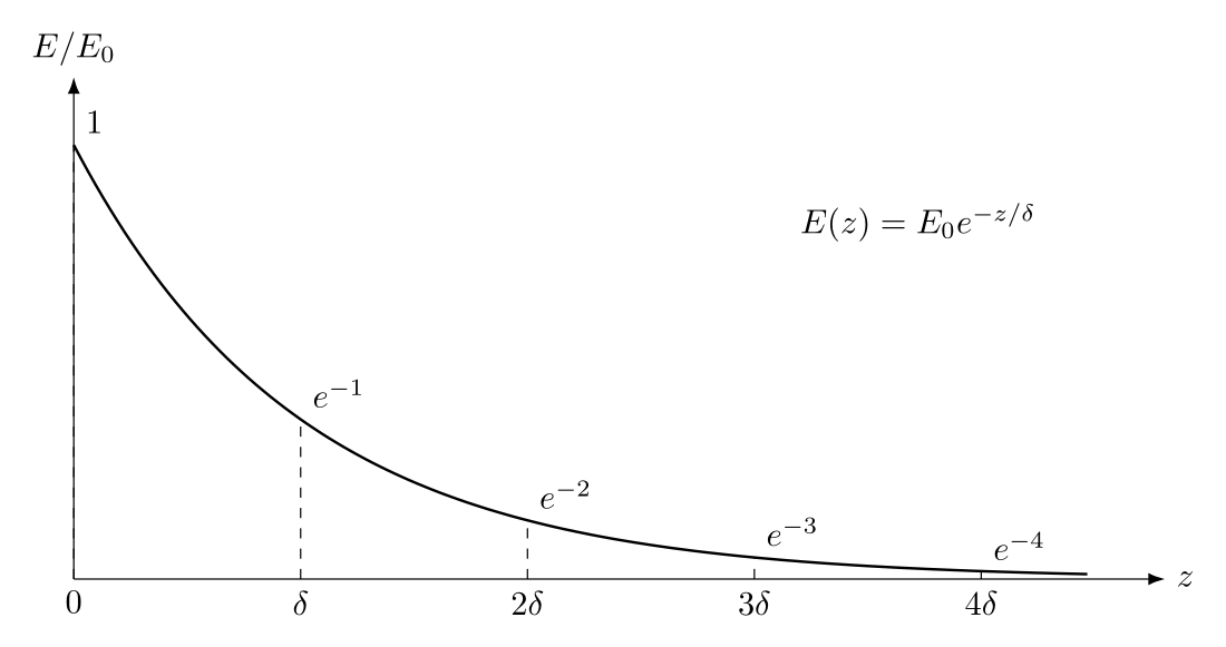
Figure 1. Field amplitude decays as e−αz while power density decays as e−2αz.
Part I: Exercises
Exercise 1: read a lossy plane waveA plane wave is written
Identify α, β, the wavelength, the phase velocity, the amplitude reduction after 3.0 m, and the power-density reduction after the same distance.
Exercise 2: lossless dielectric at 2.4 GHzA nonmagnetic lossless dielectric has
At f = 2.4 GHz, calculate
Compare the wavelength with the vacuum wavelength.
Exercise 3: attenuation in nepers and decibelsA wave propagates through a lossy medium with
After 8.0 m, determine
Explain why both the amplitude calculation using 20 log 10 and the Power calculation using 10 log 10 give the same dB loss.
Exercise 4: infer the attenuation constant from measurementsThe electric-field amplitude falls to 25% of its initial value after traveling 5.0 m in a homogeneous medium. Determine α in Np/m and the corresponding attenuation over the 5.0 m path in dB.
Exercise 5: exact lossy-dielectric propagation constantsTake
Using the exact formulas, calculate
Exercise 6: test the low-loss approximationFor the medium in Exercise 5, use
Compare each approximation with the exact result and compute the percentage error.
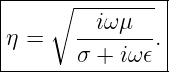
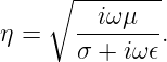
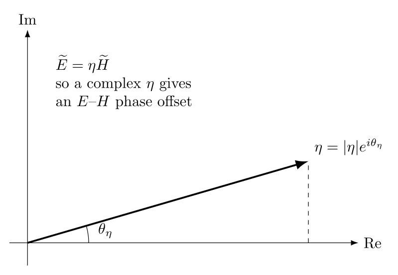
Exercise 7: complex intrinsic impedance in a lossy dielectricFor the material in Exercise 5, calculate the exact complex intrinsic impedance
Express the answer in both rectangular and polar form. If the electric-field phasor amplitude is
find the magnetic-field phasor amplitude H0 and state the phase relation between E and H.
Figure 2. A complex intrinsic impedance means the electric and magnetic phasors are not exactly in phase.
Exercise 8: impedance of a lossless high-permittivity dielectricA nonmagnetic, lossless material has 𝜖r = 9. Find its intrinsic impedance and compare it with free space. If the electric-field amplitude is 30 V/m, find the magnetic-field amplitude.
Exercise 9: copper at 1 MHzTreat copper as a good conductor with
Calculate
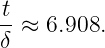
Exercise 10: frequency scaling in a good conductorFor copper, compare 1 MHz and 100 MHz. Without re-deriving the full expressions, predict how α, δ, and |η| scale with frequency. Then calculate their numerical values at 100 MHz from the 1 MHz values.
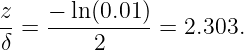
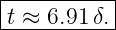
Exercise 11: how many skin depths are enough?In a good conductor the field amplitude obeys
Determine
Figure 3. Each additional skin depth multiplies field amplitude by e−1 and power by e−2.
Exercise 12: verify the good-conductor approximation for aluminumTake aluminum with
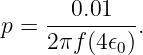
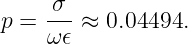
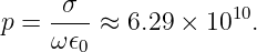
Calculate p = σ∕(ω𝜖0) and explain why the good-conductor approximation is overwhelmingly valid. Compare the approximate α with the exact α.
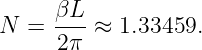
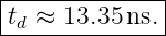
Exercise 13: phase accumulation and delay through a lossy dielectricUse the exact propagation result from Exercise 5 and let a wave travel L = 2.0 m. Find
Exercise 14: idealized conductor thickness for 60 dB field attenuationAt 10 MHz, estimate the copper thickness required for 60 dB of attenuation due only to propagation inside the conductor. Use the good-conductor approximation. Express the result in millimeters and in skin depths. State an important limitation of interpreting this number as a complete shielding calculation.
Exercise 15: derive α and β from γ2Start from
Derive the exact formulas for α and β. Then recover the limiting forms for
Exercise 16: Julia comparison of exact and approximate propagation modelsWrite a Julia program that sweeps frequency from 103 to 1010 Hz for a material with
At each frequency calculate the exact α, β, and |η|, along with the low-loss and good-conductor approximations. Plot or tabulate enough points to identify where each approximation becomes reasonable. Use the included file EM20E1_propagation_sweep.jl as a reference implementation after attempting the exercise.
Figure 4. The dimensionless ratio p = σ∕(ω𝜖) organizes the approximation hierarchy.
Part II: Complete Worked Solutions
Solution 1: read a lossy plane waveCompare
with
Therefore
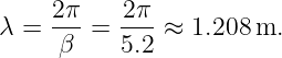
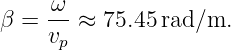
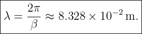
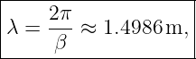
The wavelength is
The frequency is f = 108 Hz, so
Thus
At z = 3 m,
Power density is proportional to field amplitude squared, so
Hence
Solution 2: lossless dielectric at 2.4 GHzFor a lossless material,
With μr = 1 and 𝜖r = 2.25,
so
The angular frequency is
Then
Therefore
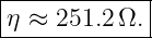
The intrinsic impedance is
Thus
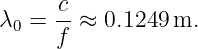
The vacuum wavelength is
The dielectric wavelength is shorter by the factor 1.5:
Solution 3: attenuation in nepers and decibelsThe amplitude ratio is
Thus
The power-density ratio is
so
Using field amplitude,
Equivalently,
Using power,
The two answers agree because power is proportional to the square of field amplitude.
Solution 4: infer the attenuation constant from measurementsWe are given
Taking natural logarithms,
Therefore
The dB attenuation is
Thus a four-to-one reduction in field amplitude corresponds to approximately 12.04 dB of attenuation.
Solution 5: exact lossy-dielectric propagation constantsThe material parameters are
First,
Since p ≪ 1, the medium is low loss, but we will use the exact formulas. The attenuation constant is
which gives
Similarly,
Then
and
After 10 m,
Thus the phase behavior is close to that of a lossless 𝜖r = 4 dielectric, while the field amplitude falls to about 39% over 10 m.
Solution 6: test the low-loss approximationFor 𝜖 = 4𝜖0 and μ = μ0,
The exact result from Exercise 5 is
Therefore
For the phase constant,
Compared with βexact ≈ 4.19275 rad/m,
The small errors confirm what the ratio p ≈ 0.0449 already suggested: the low-loss approximation is excellent here.
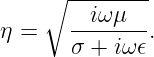
Solution 7: complex intrinsic impedance in a lossy dielectricUse
Substitution gives
The magnitude is
and the phase is
Hence
Since
we obtain
and
Therefore
With this convention, E leads H by about 1.287∘.
Solution 8: impedance of a lossless high-permittivity dielectricFor a lossless nonmagnetic material,
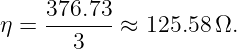
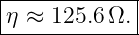
Thus
Therefore
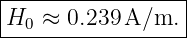
This is one third of the free-space impedance. If E0 = 30 V/m,
Hence
Solution 9: copper at 1 MHzFor a good conductor,
With f = 1 MHz, μ = μ0, and σ = 5.8 × 10⁷ S/m,
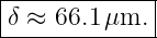
The skin depth is
so
The wavelength in the conductor is
therefore
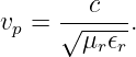
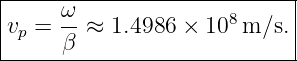
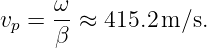
The phase velocity is
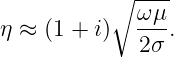
This very small phase velocity should not be confused with a signal or energy velocity in free space; the field is attenuated extremely rapidly. The good-conductor intrinsic impedance is
Numerically,
Its magnitude and phase are
Solution 10: frequency scaling in a good conductorFor fixed μ and σ,
Increasing frequency from 1 MHz to 100 MHz multiplies f by 100, so Therefore
and
The higher-frequency field penetrates less deeply even though the magnitude of the field ratio E∕H increases.
Solution 11: how many skin depths are enough?For amplitude,
Hence
Therefore
For power,
so
Thus
For copper at 1 MHz, δ ≈ 66.085 μm. Hence
and
Power reaches 1% in fewer skin depths because it depends on the square of field amplitude.
Solution 12: verify the good-conductor approximation for aluminumAt 10 MHz,
Then
Therefore
by more than ten orders of magnitude. The conduction current dominates the displacement current. The good-conductor result is
Using the exact formula gives the same value to the displayed precision:
The relative error is below 10−8% for these parameters. Thus
Solution 13: phase accumulation and delay through a lossy dielectricFrom Exercise 5,
For L = 2 m,
The number of cycles is
Hence
Modulo one full cycle, the phase is
Thus
The propagation delay is
so
Solution 14: idealized conductor thickness for 60 dB field attenuationFor copper at 10 MHz,
Therefore
For 60 dB field attenuation,
Hence
Thus
In skin depths,
Therefore
This result describes absorption associated with propagation inside an idealized bulk conductor. A complete shielding calculation must also account for reflection at interfaces, finite geometry, apertures, seams, polarization, incidence angle, and possible coupling through cables or penetrations.
Solution 15: derive α and β from γ2Start from
Expanding the left side gives
Equating real and imaginary parts,
Square both equations and add:
The left side is
Therefore
Now add this equation to
The result is
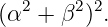
where
Hence
Similarly,
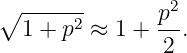
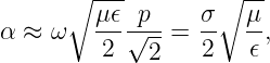
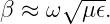
For p ≪ 1,
Then
and
Therefore
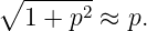
For p ≫ 1,
The ±1 terms are negligible relative to p, so
Since p = σ∕(ω𝜖),
The low-loss and good-conductor formulas are therefore limiting forms of the same exact propagation constant.
Solution 16: Julia comparison of exact and approximate propagation modelsA compact implementation should calculate
at every frequency. The exact complex quantities are
Then
For comparison, calculate
and
The included Julia script prints a logarithmically spaced table and, if Plots.jl is available, produces comparison plots. For the specified material,
The transition p ≈ 1 occurs near
Thus frequencies far below roughly 45 MHz are conductor-like for this material, while frequencies far above that scale become progressively more dielectric-like. This illustrates an important point: the propagation regime is set by both material properties and frequency.
What EM20E1 adds to the seriesEM20 introduced the propagation formulas. EM20E1 develops the calculation habits needed to use them reliably:
The next boundary-value step is to ask what happens when η changes discontinuously at an interface. That leads directly to reflection, transmission, and refraction.
References
References
[1] D. J. Griffiths, Introduction to Electrodynamics, 4th ed., Cambridge University Press, 2017. [2] D. K. Cheng, Field and Wave Electromagnetics, 2nd ed., Addison-Wesley, 1989. [3] F. T. Ulaby and U. Ravaioli, Fundamentals of Applied Electromagnetics, 7th ed., Pearson, 2015. [4] C. A. Balanis, Advanced Engineering Electromagnetics, 2nd ed., Wiley, 2012. [5] J. D. Jackson, Classical Electrodynamics, 3rd ed., Wiley, 1999. "Electromagnetic Waves, Antennas, and RF: Wave Propagation in Materials - Exercises and Complete Worked Solutions" is owned by bloftin.
This object's parent. Cross-references: displacement, conduction, energy, impedance, magnitude, parameters, square, program, Power, vacuum wavelength, velocity, Maxwell's equations, Conductor, relations, formulas, electromagnetic waves, skin depth, intrinsic impedance, phase constant, attenuation constant, propagation constant, EM20 This is version 3 of Electromagnetic Waves, Antennas, and RF: Wave Propagation in Materials - Exercises and Complete Worked Solutions, born on 2026-10-09, modified 2026-10-09. Object id is 1444, canonical name is ElectromagneticWavesAntennasAndRFWavePropagationInMaterialsExercisesAndCompleteWorkedSolutions. Accessed 12 times total. Classification:
|
|
|
|
Pending Errata and AddendaNone.
|
DiscussionNo messages.
|
Interact |
![[parent]](https://images.physicslibrary.org/images/uparrow.png)



![|----------------------------------|
| ∘ ---[∘ ---(----)-- ]1∕2 |
|α = ω μ𝜖- 1 + σ-- 2 − 1 ,|
| 2 ω𝜖 |
------------------------------------](https://images.physicslibrary.org/cache/objects/1444/make4ht/ElectromagneticWavesAntennasAndRFWavePropagationInMaterialsExercisesAndCompleteWorkedSolutions3x.png)
![|----------------------------------|
| ∘ ---[∘ ---(----)-- ]1∕2 |
|β = ω μ𝜖- 1 + σ-- 2 + 1 ,|
| 2 ω𝜖 |
------------------------------------](https://images.physicslibrary.org/cache/objects/1444/make4ht/ElectromagneticWavesAntennasAndRFWavePropagationInMaterialsExercisesAndCompleteWorkedSolutions4x.png)





























































 changes by a factor of
10.
changes by a factor of
10.
































![[∘ ------ ]
2α2 = ω2μ𝜖 1 + p2 − 1 ,](https://images.physicslibrary.org/cache/objects/1444/make4ht/ElectromagneticWavesAntennasAndRFWavePropagationInMaterialsExercisesAndCompleteWorkedSolutions126x.png)

![|------∘----[∘------------]----|
|α = ω μ𝜖- 1 + p2 − 1 1∕2 .|
| 2 |
-------------------------------](https://images.physicslibrary.org/cache/objects/1444/make4ht/ElectromagneticWavesAntennasAndRFWavePropagationInMaterialsExercisesAndCompleteWorkedSolutions128x.png)
![|------------------------------|
| ∘ -μ𝜖[∘ ------ ]1∕2 |
|β = ω --- 1 + p2 + 1 . |
----------2--------------------](https://images.physicslibrary.org/cache/objects/1444/make4ht/ElectromagneticWavesAntennasAndRFWavePropagationInMaterialsExercisesAndCompleteWorkedSolutions129x.png)