Electromagnetic Waves, Antennas, and RF: Huygens Principle and Electromagnetic Field
Equivalence
The preceding articles developed electromagnetic waves, radiation from currents, antenna gain and
effective aperture, and complete RF/ link budgets. We now return to the field itself and ask a more
structural question:
If the electric and magnetic fields are known on a surface, can the sources
behind that surface be replaced by new sources placed only on the surface, while
preserving the field everywhere on the side of interest?
The answer is yes. The result is the electromagnetic equivalence principle, one of the central ideas
behind aperture antennas, diffraction theory, reflector antennas, radomes, scattering methods, and
computational electromagnetics [2, 1, 4, 5, 3].
Its physical ancestor is Huygens’ principle: every point on a wavefront can be regarded as
launching a secondary wave, and the later wavefront is reconstructed by superposition. The scalar
Huygens picture is an extremely useful intuition, but Maxwell’s Equations sharpen it into
an exact vector statement involving equivalent electric and magnetic surface-current
densities.
The derivation chain in this article is
1 Huygens’ construction
Consider a wavefront at some instant. Huygens’ construction replaces each point on that wavefront
by a secondary source. After a short time interval, the envelope of all secondary waves forms the
next wavefront.
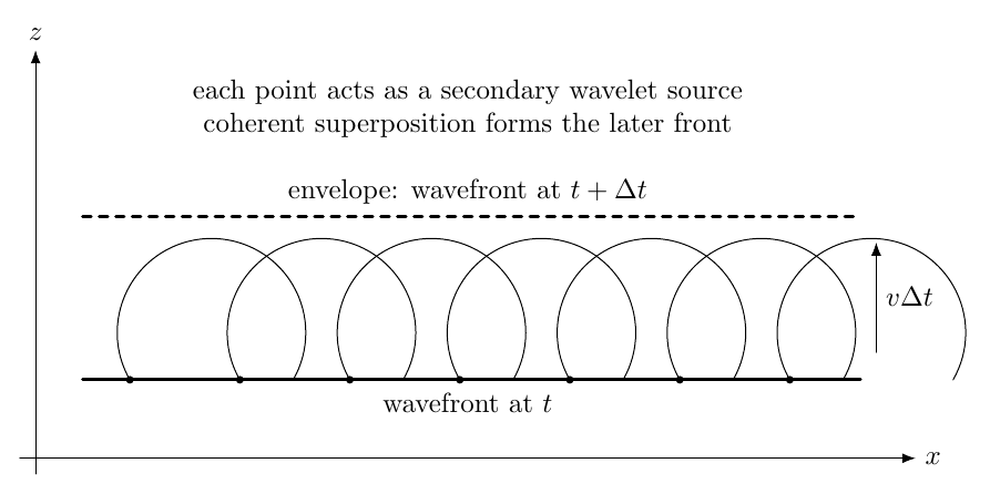
Figure. Huygens construction. Secondary wavelets emitted from points on one wavefront
combine to form a later wavefront. The construction captures propagation geometrically;
Maxwell’s equations supply the vector fields, amplitudes, polarizations, and directional
weighting.
The geometric construction already contains two ideas that will become important for
antennas:
- every point across an emitting surface contributes a wave to the observation point;
- the total field is a coherent sum, so relative phase matters as much as amplitude.
The second point is the origin of diffraction and beam formation. Different points on a finite
aperture have different path lengths to a distant observer. Their phases therefore add
constructively in some directions and destructively in others.
2 From the wave equation to a surface representation
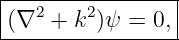
For time-harmonic fields with the convention eiωt, a scalar wave quantity ψ in a homogeneous
source-free region satisfies the Helmholtz equation
where
The outgoing-wave Green function for this convention is
It satisfies
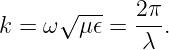
Green’s second identity then allows the value of ψ inside a closed surface S to be reconstructed
from the value of the field and its Normal derivative on that surface:
This is a mathematical form of the Huygens idea. Instead of carrying every source inside the
volume, the exterior calculation can be driven by data on the enclosing surface.
The electromagnetic problem is richer because E and H are vectors tied together by Maxwell’s curl
equations. The appropriate surface data therefore become vector surface currents rather than a
single scalar wave amplitude.
3 Surface currents and Maxwell jump conditions
Suppose a surface S separates region 1 from region 2, and let the unit normal n point from region
1 into region 2. An electric surface-current density Js has units A/m. Maxwell’s boundary
condition for the tangential magnetic field is
To write a completely symmetric field-equivalence theory, introduce a magnetic surface-current
density Ms with units V/m. It enters the tangential electric-field jump condition as
The magnetic current is a mathematical equivalent source. It does not require magnetic monopoles
to exist. It is a compact way to represent the effect of a prescribed tangential Electric Field on a
boundary [4, 5].
These two jump relations are the key to the entire equivalence principle.
4 The electromagnetic equivalence principle
Imagine a closed surface S surrounding all of the true sources. Let the original fields just outside
the surface be E and H. We now remove every true source inside the surface and replace them by
equivalent currents on S.
Choose the fields in the replacement problem to be
| E1 | = 0, | H1 | = 0 | | inside S, | (9)
|
| E2 | = E, | H2 | = H | | outside S. | (10) |
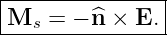
Substituting these choices into the jump conditions gives
and
These are the standard equivalent surface currents for the stated normal convention.
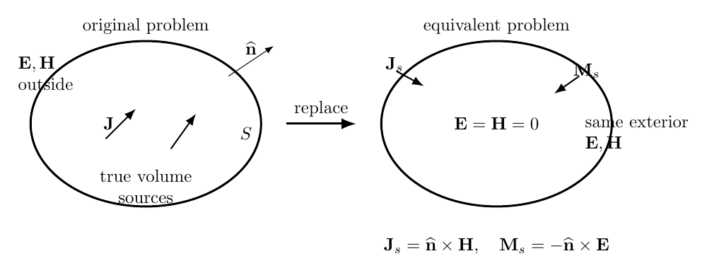
Figure. Surface equivalence. The original volume sources may be removed and replaced by
electric and magnetic currents on a closed surface. The exterior field is unchanged, while
the replacement field can be chosen to vanish inside.
This result is profound: an observer outside S cannot distinguish between the original sources and
the equivalent surface currents, because by construction both produce the same electromagnetic
field in the exterior region.
5 Love’s equivalence theorem
The special construction above is commonly called the Love equivalence principle. In its standard
exterior-field form,
The equivalent currents reproduce the original exterior field and produce zero field in the chosen
interior region, provided the replacement medium and boundary construction are defined
consistently [1, 2].
A complementary construction can preserve the interior field while forcing the exterior field to
zero. The signs reverse because the field jump is reversed. This is why equivalence-principle
formulas must always be accompanied by a stated normal direction and a clear statement of which
side is being preserved.
5.1 Why both currents are useful
If only Js were retained, it would generally be impossible to satisfy both required tangential-field
jumps simultaneously. The pair Js,Ms supplies enough freedom to recreate the desired tangential
E and H fields on the surface.
This is the vector-electromagnetic refinement of the simple Huygens picture. A Huygens surface is
not merely a sheet of scalar point sources; it carries the complete tangential field information
needed to reconstruct the electromagnetic wave.
6 Worked example: replacing a plane wave by a Huygens sheet
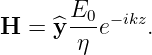
Consider a +z traveling plane wave in a lossless medium:
At the plane z = 0, choose
with the desired wave in region 2, z > 0, and zero replacement field in region 1, z < 0.
The equivalent electric surface current is
| Js | = z × | (17)
|
| = −x . . | (18) |
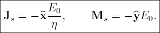
The equivalent magnetic surface current is
| Ms | = −z × (xE0) | (19)
|
| = −yE0. | (20) |
Thus
Their magnitudes satisfy
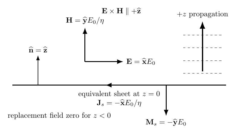
Figure. Love-equivalent sheet for a +z plane wave under the stated normal convention. The
tangential electric and magnetic fields determine orthogonal equivalent magnetic and
electric surface currents.
The paired currents form an electromagnetic Huygens source. Their relative amplitude, orientation,
and phase encode the direction in which the reconstructed field propagates.
7 Connection with the retarded Green function
EM23 showed that radiation from a localized electric-current distribution contains the
kernel
The equivalence principle does not change the propagation physics. It changes where we place the
sources. Instead of integrating through a source volume, one can integrate equivalent currents over
a surface.
Schematically, a radiated field component has the structure
The exact vector expressions contain cross products, gradients, and electric/magnetic
source terms, but the essential propagation kernel is the same outgoing spherical Green
function.
This immediately reveals the aperture-radiation problem as a coherent superposition
problem.
8 Far-field phase and the origin of beam patterns
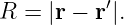
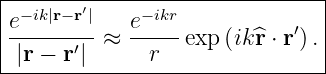
Let the observation point be far from a finite radiating surface. Write
For r ≫|r′|,
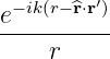
Therefore
Hence the common radial dependence factors out:
Here A(r′) stands for the appropriate weighted aperture or equivalent-current distribution.
This is the crucial bridge to the next part of the series. The angular radiation pattern is
controlled by the spatial phase transform of the field or current across the emitting
surface.
9 A one-dimensional aperture preview
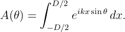
Consider a uniformly excited line aperture of width D along the x axis. In a far-field direction 𝜃,
the path-dependent phase factor is
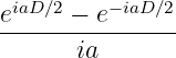
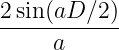
The scalar aperture factor is therefore
Let
Then
| A(𝜃) | = ![[eiax ]
----
ia](https://images.physicslibrary.org/cache/objects/1464/make4ht/ElectromagneticWavesAntennasAndRFHuygensPrincipleAndElectromagneticFieldEquivalence30x.png) −D∕2D∕2 −D∕2D∕2 | (33)
|
| =  | (34)
|
| =  . . | (35) |
Normalizing by the broadside value A(0) = D gives
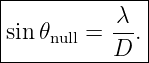
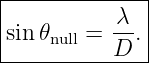
The first null occurs when
so
For
we obtain
This is only a preview. EM30 will derive aperture radiation systematically, and EM31 will make
the Fourier-transform structure explicit.
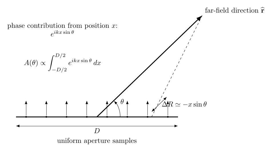
Figure. Far-field aperture geometry. Different aperture points contribute different phase
factors eikx sin 𝜃. Their coherent sum produces the angular radiation pattern.
10 Apertures in conducting screens
A practical aperture antenna often consists of an opening in a conducting surface. The fields in the
opening can be replaced by equivalent surface currents, after which the conducting
structure can be handled with an image construction or an equivalent half-space problem
[5, 4].
For a common convention with unit normal n directed into the radiating half-space, a useful
aperture-equivalence form is
where Ea is the tangential electric field in the aperture. The factor of two arises from the image
construction for the conducting plane. Other sign conventions appear in the literature
because authors may reverse the surface normal or define magnetic current with the
opposite sign. The physical field is unchanged when the complete convention is used
consistently.
This formula is one reason aperture antennas are often analyzed primarily from the electric field
distribution across the opening.
11 What Huygens’ principle does and does not say
Several distinctions are worth keeping explicit.
11.1 It is not a claim of new physical sources
Equivalent currents are a mathematical replacement. They are chosen so that Maxwell’s boundary
conditions reproduce the desired field in a specified region.
11.2 The scalar wavelet picture is not the complete electromagnetic theory
A scalar Huygens sketch suppresses polarization and vector boundary conditions. Maxwell-equivalent
electric and magnetic surface currents restore that information.
11.3 The surface can be chosen for convenience
The equivalent surface need not coincide with the physical source. A complicated antenna can be
surrounded by an imaginary closed surface, and the fields on that surface can be used as the new
source description.
11.4 Phase is fundamental
The far field is not obtained by adding surface-source magnitudes. Complex amplitudes must be
summed. A spatial phase ramp across an aperture steers the beam; an amplitude taper
changes sidelobes and beamwidth. These topics lead directly to aperture and array
theory.
12 Why this theorem is so useful
The equivalence principle connects several subjects that can otherwise seem unrelated:
- aperture antennas: replace fields across a horn or opening by equivalent sources;
- reflector antennas: replace induced aperture fields by a radiating distribution;
- diffraction: propagate known boundary fields through openings and around obstacles;
- radomes and scattering: replace complicated enclosed structures by equivalent
currents on a computational surface;
- near-field to far-field transformation: use measured tangential fields on a closed
surface to reconstruct radiation elsewhere;
- numerical electromagnetics: boundary-element and method-of-moments
formulations solve for surface currents rather than every field point in a volume.
The same logic also explains why phased arrays and continuous apertures are mathematically close
relatives. Both are distributions of coherent elementary radiators whose phases depend on
position.
13 Connection to the next articles
EM29 has established that known fields on a surface can be replaced by equivalent sources and
that the far field contains the phase factor
The next derivation is therefore natural:
EM30 develops radiation from continuous apertures. EM31 then exposes the Fourier-transform
structure explicitly, and the later array sequence discretizes the same spatial integral into a sum of
phase-weighted antenna elements.
Key results
For a surface with normal from region 1 to region 2,
For Love exterior equivalence,
In the far field,
For a uniformly excited one-dimensional aperture,
and its first null satisfies
References
References
[1] A. E. H. Love, “The integration of the equations of propagation of electric waves,”
Philosophical Transactions of the Royal Society of London A, vol. 197, pp. 1–45, 1901.
[2] S. A. Schelkunoff, “Some equivalence theorems of electromagnetics and their
application to radiation problems,” Bell System Technical Journal, vol. 15, no. 1, pp.
92–112, 1936.
[3] J. A. Stratton, Electromagnetic Theory, McGraw-Hill, 1941.
[4] R. F. Harrington, Time-Harmonic Electromagnetic Fields, IEEE Press, 2001 reissue
of the 1961 text.
[5] C. A. Balanis, Antenna Theory: Analysis and Design, 4th ed., Wiley, 2016.
[6] W. L. Stutzman and G. A. Thiele, Antenna Theory and Design, 3rd ed., Wiley,
2012.
[7] J. D. Jackson, Classical Electrodynamics, 3rd ed., Wiley, 1999.




![|----------[-------------]-----|
| ∮ ∂ψ ∂G ′|
|ψ(r) = G ---′ − ψ---′ dS .|
---------S----∂n------∂n--------](https://images.physicslibrary.org/cache/objects/1464/make4ht/ElectromagneticWavesAntennasAndRFHuygensPrincipleAndElectromagneticFieldEquivalence5x.png)











 exp
exp 












![|--------------------------|
|A (𝜃 ) = sin-[(πD--∕λ)sin𝜃-]|
| n (πD ∕λ) sin 𝜃 |
---------------------------](https://images.physicslibrary.org/cache/objects/1464/make4ht/ElectromagneticWavesAntennasAndRFHuygensPrincipleAndElectromagneticFieldEquivalence44x.png)