Calculus of Variations: The Euler–Lagrange Equation
The first four entries of this series have been building toward one result. CV00 introduced
functionals and admissible curves. CV01 made local optimality precise in function space. CV02
defined the first variation,
and showed that for
one has
CV03 proved the Fundamental Lemma: if a continuous function has zero integral against every
sufficiently localized test function, then that function must vanish pointwise.
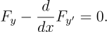
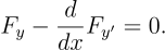
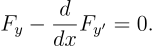
The Euler–Lagrange equation is what results when those pieces are assembled. For a stationary
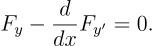
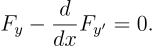
fixed-endpoint curve,
This equation is the central necessary condition of classical calculus of variations. Its importance in
physics is difficult to overstate. With the independent variable interpreted as time and F as a
Lagrangian, it becomes Lagrange’s equation of motion. With F representing arc length, optical
path, energy, or field action, the same structure generates geodesics, ray equations,
minimum-energy configurations, and field equations.
The purpose of this entry is not merely to memorize the formula. The goal is to understand exactly
why it follows, which assumptions are used, what it does and does not prove, and how to apply it
reliably.
1 Learning objectives
After this entry, the reader should be able to
- state the classical fixed-endpoint Euler–Lagrange theorem with explicit regularity
hypotheses;
- derive the theorem from local extremality, the first variation, integration by parts, and
the Fundamental Lemma;
- identify where the fixed-endpoint condition is used;
- distinguish the ordinary derivative d∕dx from the partial derivatives Fy and Fy′;
- expand the total derivative dFy′∕dx by the chain rule;
- determine when the Euler–Lagrange equation can be solved explicitly for y′′;
- use the equation to test and construct candidate extremals;
- distinguish a stationary function or extremal from a proven minimum;
- interpret the first-variation identity as a weak form and the Euler–Lagrange ODE as
a strong form under sufficient regularity;
- use the functional-derivative notation δJ∕δy correctly; and
- recognize how the surviving boundary term leads to natural boundary conditions in
CV05.
2 The entire logical chain
The Euler–Lagrange equation is not obtained by differentiating a functional in one step. The
derivation consists of a sequence of logically distinct facts.
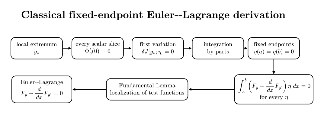
Figure. Logical chain for the classical fixed-endpoint Euler–Lagrange theorem. Each arrow
represents a separate argument: finite-dimensional Fermat stationarity, the first-variation
calculation, integration by parts, endpoint admissibility, and the Fundamental Lemma.
The chain can be summarized as
Only the forward implication is guaranteed. Solving the Euler–Lagrange equation finds stationary
candidates. It does not, by itself, prove that a candidate is a minimum.
3 Classical fixed-endpoint theorem
We now state a clean classical version. More general versions require less smoothness, but the
following hypotheses make every step of the proof transparent.
Theorem: Euler–Lagrange necessary condition. Let
where F ∈ C2 on an open set containing the values (x,y(x),y′(x)) under consideration.
Let
Suppose y∗ ∈𝒜 is a weak local minimum or weak local maximum of J. Then y∗ satisfies
for every x ∈ (a,b).
A strong local extremum also satisfies the theorem because every strong local extremum is, in
particular, a weak local extremum under the classical C0/C1 hierarchy developed in
CV01.
3.1 Why these hypotheses are convenient
The proof uses several operations:
- differentiating F(x,y + 𝜖η,y′ + 𝜖η′) with respect to 𝜖;
- differentiating Fy′(x,y∗,y∗′) with respect to x;
- integrating by parts; and
- applying the classical Fundamental Lemma to a continuous coefficient.
The assumptions F ∈ C2 and y
∗ ∈ C2 are stronger than strictly necessary, but they
ensure all four steps are classical and pointwise. Later sections explain the weaker-form
viewpoint.
4 Proof of the Euler–Lagrange theorem
The proof is short once the earlier machinery has been established, but every step has a specific
purpose.
4.1 Step 1: choose an arbitrary admissible variation
Let η ∈ C1([a,b]) satisfy
Construct the family
Because η vanishes at the endpoints,
so the perturbed family remains in the fixed-endpoint admissible class for sufficiently small
𝜖.
4.2 Step 2: reduce to an ordinary scalar extremum
Define
Because y∗ is a local extremum of J, the scalar function Φ has a local extremum at 𝜖 = 0. Ordinary
Fermat stationarity therefore gives
By definition of the first variation,
This conclusion holds for every admissible variation η.
4.3 Step 3: insert the first-variation formula
From CV02,
where the partial derivatives of F are evaluated along (x,y∗(x),y∗′(x)).
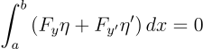
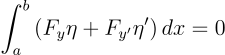
Stationarity therefore implies
for every admissible η.
4.4 Step 4: integrate by parts
The term involving η′ cannot yet be handled directly by the Fundamental Lemma because the test
function appears differentiated. Integrate that term by parts:
Thus
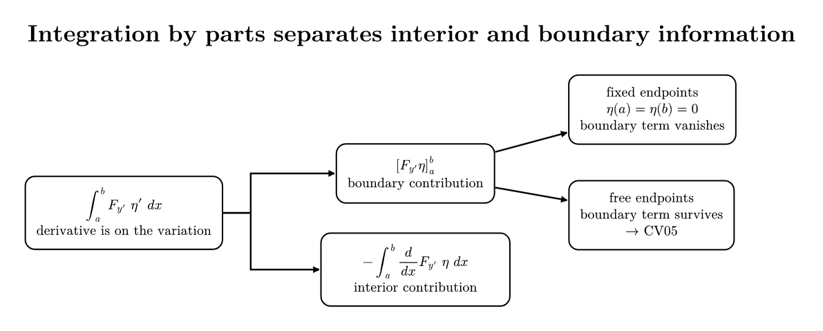
Figure. Integration by parts transfers the derivative from the arbitrary variation η onto
the coefficient Fy′. This creates both the interior Euler–Lagrange expression and a
boundary term. Fixed endpoints remove the boundary term; free endpoints will not, which
is the subject of CV05.
4.5 Step 5: use the fixed endpoints
Since
one has
Therefore stationarity reduces to
for every admissible variation η.
This is the exact point at which the fixed-endpoint assumption enters the classical proof.
4.6 Step 6: apply the Fundamental Lemma
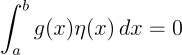
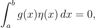
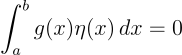
Define
Under the stated smoothness assumptions, g is continuous. The stationarity condition
says
for every admissible test function. In particular, it holds for every smooth compactly supported
test function in (a,b). The Fundamental Lemma therefore gives
for all x ∈ (a,b).
Consequently,
This completes the proof.
5 What integration by parts is really doing
The first-variation formula contains two independent pieces of perturbation data: η and η′. The
Fundamental Lemma is designed for an integral of the form
not for an expression containing both η and η′. Integration by parts reorganizes the first variation
so that the arbitrary interior perturbation appears only as η.
This is why the operation is structural rather than cosmetic. It separates the first variation
into
The interior contribution produces the Euler–Lagrange differential equation. The boundary
contribution produces endpoint conditions when the endpoints are not fixed.
This pattern reappears throughout mathematical physics. In field theory, multidimensional
integration by parts separates bulk field equations from boundary terms. In finite-element and
weak-form methods, the same operation reduces derivative requirements on the trial or test
functions.
6 Anatomy of the Euler–Lagrange equation
For
the equation is
There are two different kinds of derivative in this expression.
6.1 Partial derivative with respect to y
The quantity
means differentiate the function F(x,y,p) with respect to its second argument while holding the
other arguments fixed.
6.2 Partial derivative with respect to the slope argument
Similarly,
means differentiate F with respect to its third argument.
6.3 Total derivative along the candidate curve
After Fy′ is formed, it becomes a function of x through
Its derivative in the Euler–Lagrange equation is therefore a total derivative:
Substitution gives the expanded form
This expansion is often useful when converting the variational condition into an explicit differential
equation.
7 Regular and degenerate cases
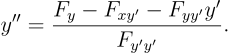
If
then locally the expanded Euler–Lagrange equation can be solved for y′′:
Such a problem is often called regular with respect to the slope variable. The Euler–Lagrange
condition is then an ordinary second-order differential equation.
If
the equation can be degenerate. It may reduce to a first-order relation or an algebraic constraint
rather than determining y′′. This is an early glimpse of the distinction between regular and
singular variational problems.
8 A reliable calculation workflow
For practical calculations it is useful to separate the operations rather than trying to write the final
differential equation from memory.
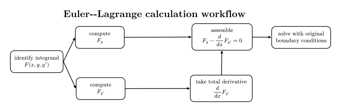
Figure. A robust Euler–Lagrange workflow. Treat F as a function of independent
arguments, compute the two required partial derivatives, take the total x-derivative only
after substituting the path dependence, and then assemble the equation.
The algorithm is
- Identify the integrand F(x,y,y′).
- Compute Fy.
- Compute Fy′.
- Compute the total derivative d(Fy′)∕dx.
- Form
- Solve the resulting differential equation subject to the original endpoint or boundary
conditions.
- After finding a stationary curve, separately ask whether it is actually a minimum, maximum,
or saddle-type stationary function.
9 Example 1: quadratic slope functional
Consider
with fixed endpoints
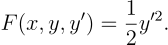
The integrand is
Therefore
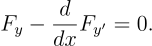
The Euler–Lagrange equation gives
so
Integrating twice,
The endpoint conditions determine the straight line
CV01 already proved directly that this curve is the global minimizer of the quadratic slope
functional. Here Euler–Lagrange recovers it as the stationary candidate.
This comparison is useful: Euler–Lagrange gives a necessary differential equation, while the direct
square-completion or convexity argument establishes actual minimality.
10 Example 2: shortest planar curve
The length of a graph y(x) between fixed x-coordinates is
Here
Since F does not depend explicitly on y,
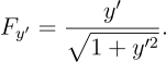
Also,
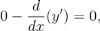
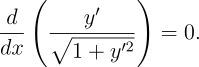
Euler–Lagrange yields
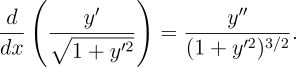
Differentiate explicitly:
Hence
and the stationary curve is again a straight line.
CV04E2 will develop this problem in more detail, including the geometric interpretation and direct
length comparison.
11 Example 3: a nonlinear integrand
Consider
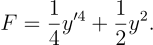
The integrand is
Therefore
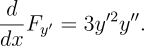
Taking the total derivative,
Thus the Euler–Lagrange equation is
This example illustrates why one should not assume that the Euler–Lagrange equation is
linear. A simple-looking integral functional can produce a highly nonlinear differential
equation.
12 Example 4: preview of classical mechanics
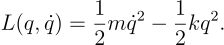
Let the independent variable be time t and consider the harmonic-oscillator action
with
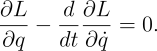
The Euler–Lagrange equation is now written
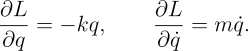
Compute
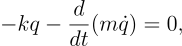
Therefore
or
Thus the familiar differential equation for a harmonic oscillator is itself an Euler–Lagrange
equation. CV14 will derive the full connection between Hamilton’s principle and Lagrange’s
equations for many-degree-of-freedom mechanical systems.
13 Necessary does not mean sufficient
The theorem says
The converse is false in general.
A solution of the Euler–Lagrange equation is commonly called an extremal in classical terminology,
even though it may not actually be a minimum or maximum. To avoid ambiguity, it is often
helpful to say stationary extremal or Euler–Lagrange extremal when classification has not yet been
established.
13.1 Stationary maximum
Consider
with y(0) = y(1) = 0. The Euler–Lagrange equation is again
so the only endpoint-compatible stationary curve is y = 0. But now
for every admissible y. Thus y = 0 is a global maximum, not a minimum.
13.2 Stationary saddle-type example
Consider
with y(0) = y(1) = 0. The zero function satisfies the Euler–Lagrange equation and is
stationary.
Now compare the two admissible directions
For y = 𝜖η1,
when 𝜖≠0, while for y = 𝜖η2,
Therefore arbitrarily close admissible curves exist with both larger and smaller values of J. The
stationary curve y = 0 is saddle-type.
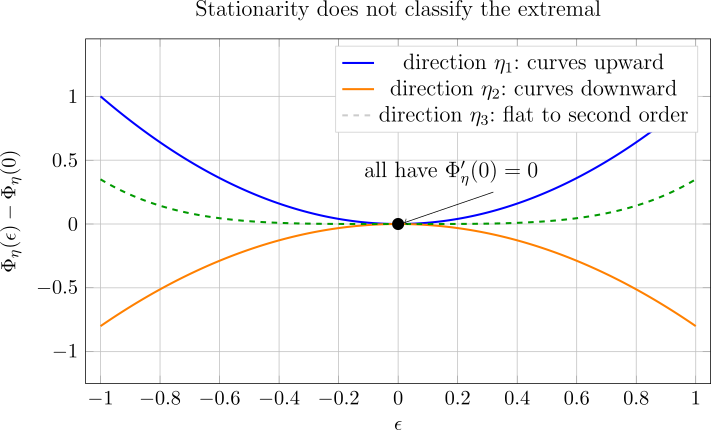
Figure. Vanishing first variation means that every one-dimensional slice Φη(𝜖) = J[y∗ + 𝜖η] has
zero slope at 𝜖 = 0. It does not determine the curvature of those slices. Different directions can
bend upward, downward, or remain flat to second order, so stationarity alone does not classify the
extremal.
Second-variation theory begins in CV11 precisely because this classification question requires
additional information.
14 Weak form and strong form
Before applying the Fundamental Lemma, stationarity can be written as
for every admissible test function η. This is a variational or weak-form statement.
After integration by parts and sufficient regularity, the Fundamental Lemma produces the
pointwise differential equation
This is the corresponding classical strong form.
In modern analysis, a function may satisfy the weak variational identity even when it does not
possess enough classical derivatives for the strong equation to make pointwise sense. Under
additional regularity, weak solutions can often be shown to satisfy the strong equation. This
weak-to-strong relationship is a major bridge from the calculus of variations to partial differential
equations and finite-element methods.
15 Functional derivative notation
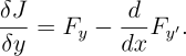
For a first-order functional, one often writes
Then the first variation may be represented schematically as
when the appropriate boundary term vanishes.
The notation is useful, but it hides the integration-by-parts step. In full,
Thus the functional derivative captures the interior coefficient of the variation. Boundary
conditions must still be handled separately.
This distinction becomes essential in CV05, field theory, and Hamiltonian mechanics.
16 Why endpoint conditions are not bookkeeping
The fixed-endpoint proof used
only after integration by parts. If an endpoint is free, the term
does not automatically vanish.
Stationarity must then control both the interior integral and the boundary contribution. The
interior still yields the Euler–Lagrange equation, while the boundary term yields a natural
boundary condition. If an endpoint is allowed to move along a prescribed curve, still more general
transversality conditions appear.
This is why the admissible class introduced in CV01 is part of the theorem itself. Changing the
endpoint freedom changes the necessary conditions.
17 Dimensional consistency
In physical applications the two terms of the Euler–Lagrange equation must have the same
dimensions.
If x has dimensions [x], y has dimensions [y], and F has dimensions [F], then
Since
one has
Taking d∕dx gives
matching [Fy]. This provides a quick error check in mechanics, optics, and engineering
applications.
18 Common mistakes
18.1 Mistake 1: using a partial derivative where a total derivative is required
The equation contains
not merely ∂Fy′∕∂x. The quantity Fy′ also changes because y(x) and y′(x) change.
18.2 Mistake 2: dropping the boundary term before integrating by parts
The boundary term must first be produced. It vanishes only because of the specific endpoint
conditions of the problem.
18.3 Mistake 3: treating y′ as dependent on y when computing partial derivatives
When computing Fy and Fy′, treat x, y, and y′ as independent arguments of F. Their path
dependence is reintroduced when taking the total x-derivative.
18.4 Mistake 4: believing every Euler–Lagrange solution is a minimum
Euler–Lagrange is a stationarity condition. A stationary curve can be a minimum, maximum, or
saddle-type extremal.
18.5 Mistake 5: forgetting the original endpoint conditions
The differential equation produces a family of candidate solutions. The original boundary data
select the admissible members of that family.
18.6 Mistake 6: cancelling the variation from the integral
From
one cannot algebraically cancel η. The conclusion g = 0 follows from the Fundamental Lemma and
the richness of the test-function class.
18.7 Mistake 7: confusing existence with stationarity
Even if the Euler–Lagrange boundary-value problem has a formal solution, a minimizer of the
original variational problem need not exist under arbitrary hypotheses. Existence is a separate
question involving compactness, coercivity, and lower semicontinuity in more advanced
theory.
19 A compact theorem checklist
When using Euler–Lagrange, ask the following questions.
- What is the admissible class?
- Are the endpoints fixed or free?
- Is the candidate regular enough for the classical theorem?
- What is the integrand F(x,y,y′)?
- What are Fy and Fy′?
- Did I take a total derivative of Fy′?
- What boundary conditions must the resulting ODE satisfy?
- Have I shown only stationarity, or have I actually proved minimality?
Keeping these questions separate prevents most common variational mistakes.
20 What CV05 and CV06 add
CV04 has used fixed endpoints to eliminate the boundary term
CV05 removes that simplification. Free endpoints, movable endpoints, and endpoints constrained
to curves produce natural boundary and transversality conditions.
CV06 then studies special forms of the Euler–Lagrange equation. If the integrand lacks explicit
dependence on certain variables, the differential equation admits first integrals such as the
Beltrami identity. These conservation-like reductions are especially important in the catenary,
brachistochrone, mechanics, and optics.
21 Summary
For the classical fixed-endpoint functional
a sufficiently smooth local extremum must satisfy the Euler–Lagrange equation
The derivation is
Integration by parts separates boundary and interior behavior. Fixed endpoints remove the
boundary term, while the Fundamental Lemma converts the remaining integral identity into a
pointwise differential equation.
The resulting equation is a necessary condition for stationarity, not a proof of minimality.
Classification, existence, boundary freedom, conservation laws, and physical specialization all
require additional theory developed in the following entries.
22 References and further reading
- I. M. Gelfand and S. V. Fomin, Calculus of Variations.
- B. van Brunt, The Calculus of Variations.
- C. Fox, An Introduction to the Calculus of Variations.
- C. Lanczos, The Variational Principles of Mechanics.
- H. Goldstein, C. Poole, and J. Safko, Classical Mechanics.
- L. C. Evans, Partial Differential Equations, for weak formulations and the modern
variational viewpoint.

![|
δJ[y;η] = -dJ [y + 𝜖η ]|| ,
d𝜖 |𝜖=0](https://images.physicslibrary.org/cache/objects/1140/make4ht/CalculusOfVariationsTheEulerLagrangeEquation0x.svg)
![∫ b
J[y] = F (x,y,y′)dx,
a](https://images.physicslibrary.org/cache/objects/1140/make4ht/CalculusOfVariationsTheEulerLagrangeEquation1x.svg)
![∫ b
δJ[y;η] = (Fy η + Fy′η ′)dx.
a](https://images.physicslibrary.org/cache/objects/1140/make4ht/CalculusOfVariationsTheEulerLagrangeEquation2x.svg)
![local extremum =⇒ δJ[y;η] = 0 for every admissible η =⇒ integral identity = ⇒ Euler–Lagrange equation.](https://images.physicslibrary.org/cache/objects/1140/make4ht/CalculusOfVariationsTheEulerLagrangeEquation4x.svg)
![∫ b
J[y] = F (x,y,y′)dx,
a](https://images.physicslibrary.org/cache/objects/1140/make4ht/CalculusOfVariationsTheEulerLagrangeEquation5x.svg)
![{ 2 }
𝒜 = y ∈ C ([a,b]) : y (a) = A, y(b) = B .](https://images.physicslibrary.org/cache/objects/1140/make4ht/CalculusOfVariationsTheEulerLagrangeEquation6x.svg)




![Φ (𝜖) = J [y∗ + 𝜖η].](https://images.physicslibrary.org/cache/objects/1140/make4ht/CalculusOfVariationsTheEulerLagrangeEquation11x.svg)

![δJ [y∗;η ] = 0.](https://images.physicslibrary.org/cache/objects/1140/make4ht/CalculusOfVariationsTheEulerLagrangeEquation13x.svg)
![∫ b
δJ [y ∗;η ] = (Fyη + Fy′η′)dx,
a](https://images.physicslibrary.org/cache/objects/1140/make4ht/CalculusOfVariationsTheEulerLagrangeEquation14x.svg)
![∫ ∫
b ′ b b d--
Fy ′η dx = [Fy′η ]a − dxFy ′ ηdx.
a a](https://images.physicslibrary.org/cache/objects/1140/make4ht/CalculusOfVariationsTheEulerLagrangeEquation16x.svg)
![∫ ( )
b b d--
δJ [y∗;η ] = [Fy′η]a + Fy − dxFy ′ η dx.
a](https://images.physicslibrary.org/cache/objects/1140/make4ht/CalculusOfVariationsTheEulerLagrangeEquation17x.svg)

![b
[Fy′η]a = 0.](https://images.physicslibrary.org/cache/objects/1140/make4ht/CalculusOfVariationsTheEulerLagrangeEquation19x.svg)












![1 ∫ b
J [y] = -- y′(x)2 dx
2 a](https://images.physicslibrary.org/cache/objects/1140/make4ht/CalculusOfVariationsTheEulerLagrangeEquation38x.svg)





![∫ b∘ -------
J [y ] = 1 + y′2 dx.
a](https://images.physicslibrary.org/cache/objects/1140/make4ht/CalculusOfVariationsTheEulerLagrangeEquation46x.svg)



![∫ b( )
J[y] = 1y ′4 + 1y2 dx.
a 4 2](https://images.physicslibrary.org/cache/objects/1140/make4ht/CalculusOfVariationsTheEulerLagrangeEquation53x.svg)


![∫
t2
S[q] = L (q, ˙q,t)dt,
t1](https://images.physicslibrary.org/cache/objects/1140/make4ht/CalculusOfVariationsTheEulerLagrangeEquation58x.svg)


![∫
1 ′2
J[y] = − y dx
0](https://images.physicslibrary.org/cache/objects/1140/make4ht/CalculusOfVariationsTheEulerLagrangeEquation65x.svg)

![J [y] ≤ 0 = J [0]](https://images.physicslibrary.org/cache/objects/1140/make4ht/CalculusOfVariationsTheEulerLagrangeEquation67x.svg)
![∫ 1( ′2 2 2)
J[y] = y − 2π y dx
0](https://images.physicslibrary.org/cache/objects/1140/make4ht/CalculusOfVariationsTheEulerLagrangeEquation68x.svg)

![π2
J [𝜖η1] = − --𝜖2 < 0
2](https://images.physicslibrary.org/cache/objects/1140/make4ht/CalculusOfVariationsTheEulerLagrangeEquation70x.svg)
![J[𝜖η2] = π2𝜖2 > 0.](https://images.physicslibrary.org/cache/objects/1140/make4ht/CalculusOfVariationsTheEulerLagrangeEquation71x.svg)
![∫
bδJ-
δJ [y;η ] = δy η dx
a](https://images.physicslibrary.org/cache/objects/1140/make4ht/CalculusOfVariationsTheEulerLagrangeEquation76x.svg)
![∫ b
δJ [y; η] = [Fy′η]b+ δJ-η dx.
a a δy](https://images.physicslibrary.org/cache/objects/1140/make4ht/CalculusOfVariationsTheEulerLagrangeEquation77x.svg)

![b
[Fy′η]a](https://images.physicslibrary.org/cache/objects/1140/make4ht/CalculusOfVariationsTheEulerLagrangeEquation79x.svg)
![[F-]
[Fy] = [y] .](https://images.physicslibrary.org/cache/objects/1140/make4ht/CalculusOfVariationsTheEulerLagrangeEquation80x.svg)
![′ [y]
[y ] = [x],](https://images.physicslibrary.org/cache/objects/1140/make4ht/CalculusOfVariationsTheEulerLagrangeEquation81x.svg)
![[F ][x]
[Fy ′] = ------.
[y]](https://images.physicslibrary.org/cache/objects/1140/make4ht/CalculusOfVariationsTheEulerLagrangeEquation82x.svg)
![[ d ] [F ]
---Fy′ = ----,
dx [y ]](https://images.physicslibrary.org/cache/objects/1140/make4ht/CalculusOfVariationsTheEulerLagrangeEquation83x.svg)

![[Fy′η ]ba .](https://images.physicslibrary.org/cache/objects/1140/make4ht/CalculusOfVariationsTheEulerLagrangeEquation86x.svg)
![∫
b ′
J[y] = F (x,y,y )dx,
a](https://images.physicslibrary.org/cache/objects/1140/make4ht/CalculusOfVariationsTheEulerLagrangeEquation87x.svg)