Celestial Mechanics: Central Forces and Conservation Laws
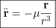
CM03 reduced Newtonian two-body gravitation to the relative equation
For a spacecraft or other negligible test mass moving about a much larger body, the
usual approximation is  . Equation (1) is already enough to reveal two of the
deepest structural properties of Keplerian motion: conservation of angular momentum and
conservation of mechanical energy. From those two constants follow planarity, constant areal
velocity, the distinction between bound and unbound motion, the circular-orbit and
escape-speed scales, and much of the orbit classification used throughout celestial mechanics
[1, 2, 3, 4].
. Equation (1) is already enough to reveal two of the
deepest structural properties of Keplerian motion: conservation of angular momentum and
conservation of mechanical energy. From those two constants follow planarity, constant areal
velocity, the distinction between bound and unbound motion, the circular-orbit and
escape-speed scales, and much of the orbit classification used throughout celestial mechanics
[1, 2, 3, 4].
This article derives those results directly from Newton’s orbital equation. The purpose is not to
memorize orbital formulas, but to see why they exist.
1. Central forces
A force is called central when it always acts along the instantaneous radius vector joining the
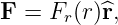
particle to a fixed force center. The most general central force may be written
where  is a signed scalar. An attractive force has
  . Newtonian gravity
has
. Newtonian gravity
has
The defining geometric fact is therefore
That simple parallelism is what produces angular-momentum conservation.
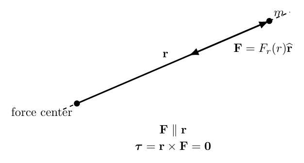
Figure 1. For a central force,  is parallel or antiparallel to
  . The moment arm
about the force center is therefore zero, so the torque vanishes identically.
. The moment arm
about the force center is therefore zero, so the torque vanishes identically.
2. Torque and angular momentum
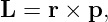
For a particle of mass  , define the angular momentum about the force center as
with linear momentum
Thus
The torque about the origin is
Differentiate  :
:
 | =  (r × mv) (r × mv) | (9)
|
| = r × mv + r × mv. | (10) |
Because  , the first term is
Newton’s second law gives  , so
, so
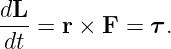
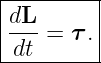
This is the angular form of Newton’s second law:
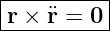
For a central force,
because  and
and  are parallel. Therefore
and hence
This result applies to every central force, not only inverse-square gravity.
3. Specific angular momentum
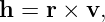
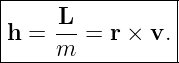
In celestial mechanics it is convenient to divide angular momentum by the orbiting mass. Define
the specific angular momentum
Because  is constant,
The SI units of  are
are
In astrodynamics,  is commonly used.
The magnitude of the cross product is
where  is the angle between
  and
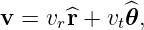
and  . If the velocity is decomposed into radial and
transverse parts,
. If the velocity is decomposed into radial and
transverse parts,
then only the transverse velocity contributes:
Purely radial motion has  , and therefore
4. Why a central-force orbit is planar
For any instant of motion,
A cross product is perpendicular to both of its factors. Therefore
and
If  and is constant, then the radius vector must always remain in the fixed plane through
the origin perpendicular to
and is constant, then the radius vector must always remain in the fixed plane through
the origin perpendicular to  . Consequently,
The original three-dimensional differential equation can therefore be reduced once the fixed orbital
plane is known. The remaining motion is two-dimensional.
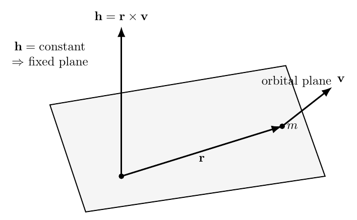
Figure 2. The conserved vector  is normal to the orbital plane. Because its
direction does not change, the plane itself remains fixed in the ideal central-force problem.
is normal to the orbital plane. Because its
direction does not change, the plane itself remains fixed in the ideal central-force problem.
The radial case  is degenerate. There is then no unique orbital-plane normal because the
motion lies along a single line through the force center.
is degenerate. There is then no unique orbital-plane normal because the
motion lies along a single line through the force center.
5. Two-body meaning of the relative angular momentum
For the exact two-body problem, CM03 introduced the center-of-mass coordinate and the relative
coordinate
In the center-of-mass frame,
Solving for the individual position vectors gives
The corresponding velocities are
The total angular momentum about the center of mass is
Substitution and collection of terms gives
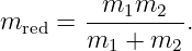
Define the reduced mass
Then
Thus  is a specific angular momentum associated with the relative orbit, while the
physical total orbital angular momentum carries the additional reduced-mass factor. In the
test-particle limit
is a specific angular momentum associated with the relative orbit, while the
physical total orbital angular momentum carries the additional reduced-mass factor. In the
test-particle limit  , the reduced mass approaches
  , recovering the familiar
 .
.
6. Areal velocity
Angular momentum has a direct geometric interpretation. During a short interval  , the particle
moves through
, the particle
moves through
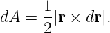
The radius vector sweeps out an approximately triangular area
Substitute  :
:
| dA | =  |r × v|dt |r × v|dt | (38)
|
| =  dt. dt. | (39) |
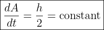
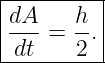
Divide by  :
:
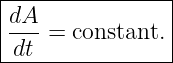
Since  is constant,
This is Kepler’s second law: equal areas are swept out in equal times. Newtonian mechanics
therefore explains Kepler’s empirical area law as a direct consequence of zero torque about the
force center.
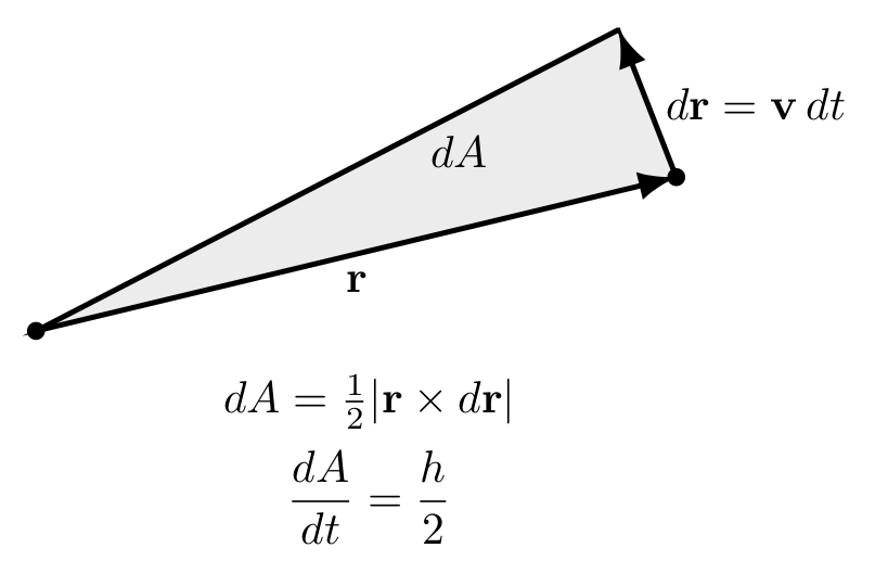
Figure 3. In a short interval  , the swept area is
  . Conservation of
 therefore makes the areal velocity constant.
7. Polar-coordinate form of angular momentum
In the orbital plane,
Then
| h | = rer ×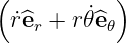 | (43)
|
| = r2𝜃 . . | (44) |
Thus
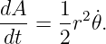
The areal-velocity relation becomes
This form will be used in CM05 and CM06 to reduce the two-dimensional central-force problem to
a radial equation and then to Binet’s equation.
8. Mechanical energy from the gravitational potential
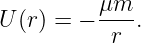
CM02 derived the Newtonian gravitational potential energy
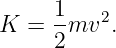
The kinetic energy is
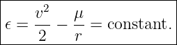
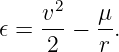
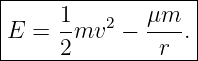
Therefore the total mechanical energy is
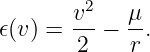
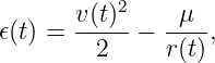
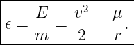
Dividing by the particle mass gives the specific mechanical energy
Its units are
9. Direct derivation of energy conservation from Newton’s equation
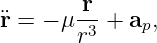
We can prove energy conservation without first assuming the potential-energy formula. Start from
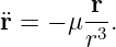
Newton’s orbital equation
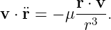
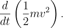
Take the dot product with the velocity  :
:
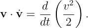
The left side is
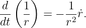
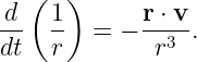
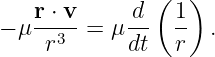
For the gravitational term, note that
Also,
Therefore
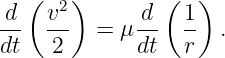
Hence
Substituting into the dot-product equation gives
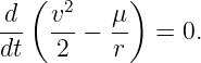
Bring both derivatives to the same side:
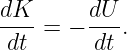
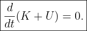
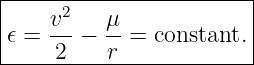
Thus
This is the specific-energy integral of the Newtonian two-body equation.
10. General central conservative forces
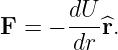
The conservation argument is broader than gravity. Suppose a central force can be derived from a
radial potential energy  :
:
Newton’s second law is
Dot with  :
:
The left side is
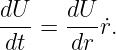
Because a central potential depends only on  ,
,
Also  , so
, so
Therefore
A central force guarantees angular-momentum conservation because its torque is zero. Energy
conservation additionally requires that the force be conservative. Newtonian gravity satisfies both
conditions.
11. The same result from work and potential energy
The work-energy theorem states
For a conservative gravitational force,
Therefore
so
The force-law derivation and the work-potential derivation are two descriptions of the same
conservation law.
12. Why angular momentum and energy are independent pieces of information
The specific energy depends on the speed magnitude:
Specific angular momentum depends only on the transverse part of velocity:
Two particles at the same  with the same speed
  therefore have the same
  , but may have
different
, but may have
different  if their velocity directions differ.
For example, a purely transverse velocity gives
whereas a purely radial velocity gives
although the two states have the same kinetic energy if their speeds are equal.
Thus:
Later, CM06 will show that together  and
and  determine the size and shape of the Kepler
conic.
determine the size and shape of the Kepler
conic.
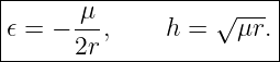
13. Energy scale at a given radius
At a fixed radius  , the specific energy is
Three speed scales are especially useful.
11.1 Zero speed
If  , then
11.2 Circular speed
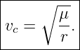
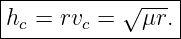
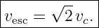
For circular motion, the inward gravitational acceleration must equal the centripetal
acceleration:
Therefore
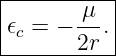
Substitute this into the energy equation:
Thus
The corresponding angular momentum magnitude is
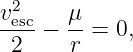
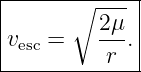
11.3 Escape speed
The minimum escape trajectory has zero speed at infinity and therefore zero total specific
energy:
At the launch radius,
so
Therefore
14. Orbit classification from specific energy
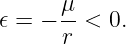
Because the gravitational potential approaches zero as  , the sign of
  has an immediate
physical meaning.
has an immediate
physical meaning.
12.1 Negative energy: bound motion
If
then the particle does not have enough mechanical energy to reach infinity with nonnegative
kinetic energy. The motion is gravitationally bound.
For  , the eventual Kepler conic is an ellipse; a circle is the special constant-radius case.
CM06 derives that conic result from Binet’s equation. If
, the eventual Kepler conic is an ellipse; a circle is the special constant-radius case.
CM06 derives that conic result from Binet’s equation. If  , the bound motion is a degenerate
radial trajectory rather than a nondegenerate ellipse.
, the bound motion is a degenerate
radial trajectory rather than a nondegenerate ellipse.
12.2 Zero energy: marginal escape
If
then the object is exactly at the escape threshold. It can reach infinity with speed tending to
zero.
For  , the corresponding Kepler conic is a parabola. For
  , the motion is radial
marginal escape.
, the motion is radial
marginal escape.
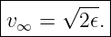
12.3 Positive energy: unbound motion
If
then the motion is unbound. At very large distance the potential term vanishes, so
Therefore
For  , CM06 shows that the Kepler conic is a hyperbola. For
  , the motion is radial
unbound motion.
, the motion is radial
unbound motion.
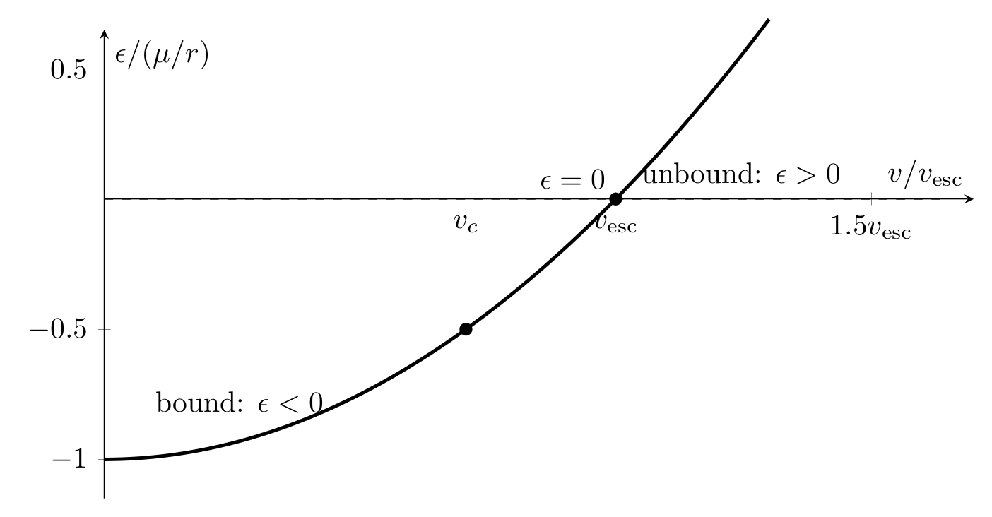
Figure 4. At a fixed radius, the sign of  separates bound,
marginal-escape, and unbound motion. The circular speed lies below the escape speed by
the factor
separates bound,
marginal-escape, and unbound motion. The circular speed lies below the escape speed by
the factor  .
.
15. Compact classification table
The two invariants  and
and  already organize the major cases:
The conic labels in this table are established formally in CM06. At the present stage, the
bound-versus-unbound classification follows directly from energy conservation.
A further consequence of angular-momentum conservation can already be obtained without
knowing the conic equation. At any radial turning point the radial speed vanishes, so the velocity
is purely transverse and
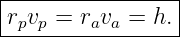
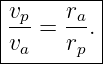
If a bound orbit has an inner turning radius  and an outer turning radius
  ,
then
,
then
Therefore
The body moves fastest at its smaller turning radius and slowest at its larger turning radius. This
is the speed counterpart of constant areal velocity.
16. Circular motion as a special simultaneous condition
Negative energy alone does not imply a circular orbit. Circular motion requires both
and the exact transverse speed
Equivalently, a circular state at radius  satisfies
A state at the same radius with the same negative energy but a different angular momentum is not
circular.
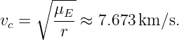
17. Example: a circular low-Earth orbit
Take
and an orbital altitude of  above a mean Earth radius
The orbital radius is
The circular speed is
The escape speed at the same radius is
The circular specific angular momentum is
The specific energy is
Thus a low-Earth satellite is deeply inside Earth’s gravitational well even though it is continuously
falling around the planet.
18. Example: classify a Cartesian initial state
Consider the state
Using Earth-centered units of km and s,
The radius and speed magnitudes are approximately
The specific energy is
Therefore the motion is bound.
The specific angular momentum is
which gives approximately
Its nonzero magnitude confirms that this is a nonradial planar orbit. The vector  supplies the
fixed normal to that orbital plane.
supplies the
fixed normal to that orbital plane.
CM06 will use these same invariants to determine the eccentricity and complete conic
geometry.
19. Conservation laws as numerical diagnostics
Conservation laws are not only analytical tools. They are also excellent diagnostics for numerical
orbit propagation.
For an ideal two-body simulation, evaluate at every numerical time step
and
Ideally,
In an actual numerical integrator, small deviations measure numerical error. A propagator may
appear visually plausible while slowly drifting in energy or angular momentum. Monitoring the
invariants makes such errors visible.
For perturbed motion, the invariants need not remain constant physically. Their rates of
change then contain information about the perturbing force rather than merely numerical
error.
20. What changes when the force is not perfectly central?
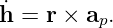
Suppose
where  is a perturbing acceleration. Then
A perturbation with a nonzero moment about the central body can therefore change both
the magnitude and direction of  , altering the orbital plane or angular-momentum
magnitude.
, altering the orbital plane or angular-momentum
magnitude.
Likewise,
when  is defined using only the central
  potential. A perturbation doing positive work
increases the Keplerian specific energy; one doing negative work decreases it.
potential. A perturbation doing positive work
increases the Keplerian specific energy; one doing negative work decreases it.
These relations foreshadow the later perturbation and variation-of-elements sections of the CM
series.
21. The conservation-law spine of the Kepler problem
The logic developed in CM03 and CM04 can now be summarized compactly:
implies
and therefore
That immediately gives
and a fixed orbital plane.
Taking the dot product with  gives
gives
The sign of  separates bound, marginal, and unbound motion. The pair
  is therefore the
natural bridge from Newton’s differential equation to orbit geometry.
is therefore the
natural bridge from Newton’s differential equation to orbit geometry.
The next steps of the course exploit exactly that bridge:
followed by
References
References
[1] I. Newton, The Principia: Mathematical Principles of Natural Philosophy, translated
by I. B. Cohen and A. Whitman, University of California Press, 1999.
[2] H. Goldstein, C. Poole, and J. Safko, Classical Mechanics, 3rd ed., Addison-Wesley,
2001.
[3] J. M. A. Danby, Fundamentals of Celestial Mechanics, 2nd ed., Willmann-Bell, 1988.
[4] R. R. Bate, D. D. Mueller, and J. E. White, Fundamentals of Astrodynamics, Dover
reprint, 1971.
[5] B. W. Carroll and D. A. Ostlie, An Introduction to Modern Astrophysics, 2nd ed.,
Pearson, 2007.












![[h] = m2 ∕s.](https://images.physicslibrary.org/cache/objects/1277/make4ht/CelestialMechanicsCentralForcesAndConservationLaws31x.png)

















![2 2
[𝜖] = m ∕s = J∕kg.](https://images.physicslibrary.org/cache/objects/1277/make4ht/CelestialMechanicsCentralForcesAndConservationLaws83x.png)