Electromagnetic Waves, Antennas, and RF: Wave Propagation in Materials
EM16 derived the electromagnetic wave equation in vacuum. EM17 and EM18 showed that the
wave transports energy and momentum, and EM19 described the geometry of its transverse
polarization. We now ask what changes when the wave travels through matter rather than empty
space.
The answer is controlled by three material parameters:
where 𝜖 is permittivity, μ is permeability, and σ is electrical conductivity. These quantities
determine how rapidly phase advances, how strongly amplitude decays, and how the electric and
magnetic fields are related [1, 2, 3, 4].
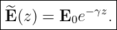
The central result is that a time-harmonic plane wave propagating in the +z direction through a
homogeneous linear medium has the form
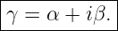
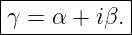
with the complex propagation constant
The real part α controls attenuation. The imaginary part β controls phase propagation.
1 Constitutive relations connect fields to material response
In a homogeneous, linear, isotropic material,
The first two equations describe electric and magnetic material response. The third is Ohm’s law in
local field form.
It is often useful to write
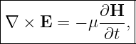
2 Maxwell’s curl equations inside the medium
In a source-free homogeneous propagation region,
and
The conduction-current density and displacement-current density are
For a sinusoidal field, the ratio of their characteristic magnitudes is
Thus
3 Derivation of the wave equation in matter
Take the curl of Faraday’s law:
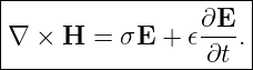
Insert the Ampere-Maxwell law:
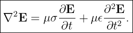
For constant material parameters,
Use
In a homogeneous source-free region,
Therefore
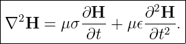
Similarly,
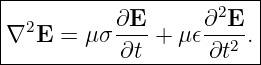
The term proportional to σ is the key addition relative to the vacuum wave equation. It produces
attenuation because electromagnetic energy is transferred to the material.
4 The lossless dielectric limit
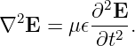
Set σ = 0. Then
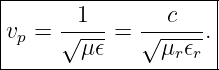
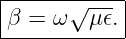
Comparison with the standard wave equation gives
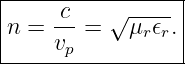
For a nondispersive lossless medium, the refractive index is
For many ordinary RF dielectrics, μr ≈ 1, so
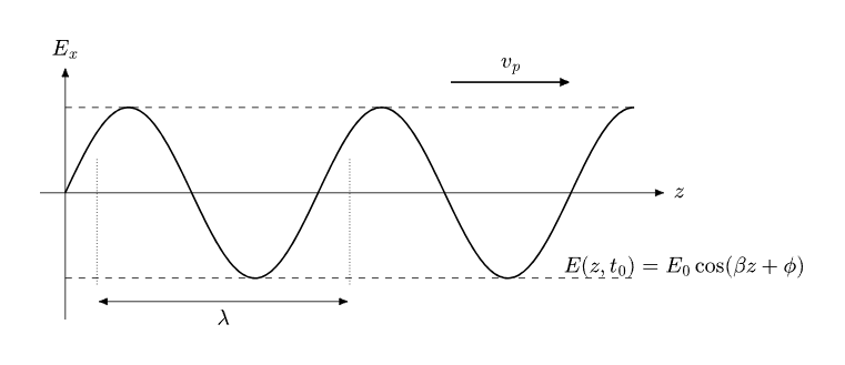
Figure 1. A lossless plane wave propagates without amplitude decay. The phase advances by
2π over one wavelength λ.
5 Frequency, wavelength, and phase constant
A sinusoidal plane wave may be written
One wavelength corresponds to a phase change of 2π, so
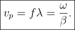
The phase velocity is
In a lossless material,
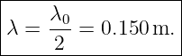
6 Example: wavelength in a lossless dielectric
Let
Then
At
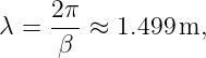
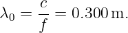
the vacuum wavelength is approximately
Inside the dielectric,
The frequency is fixed by the source; the material changes propagation speed and therefore
wavelength.
7 Time-harmonic fields and phasors
Adopt the time convention
Write
Then
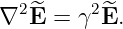
The field equation becomes
Define
Then
For one-dimensional propagation in +z,
8 The propagation constant separates attenuation and phase
Write
Then
The physical field is
Thus
The units are
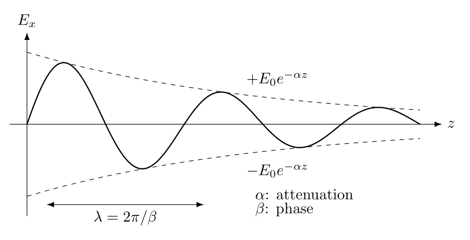
Figure 2. In a lossy medium, the sinusoid propagates while its amplitude envelope decays as
e−αz.
9 Exact attenuation and phase constants
Let
From
the real and imaginary parts give
and
Solving gives
and
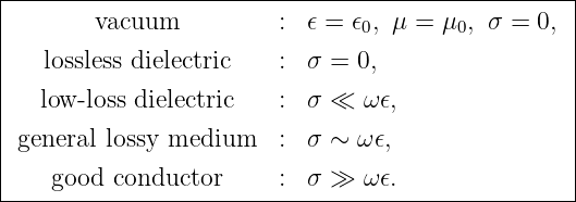
10 A material-regime map
The ratio
compares conduction current with displacement current.
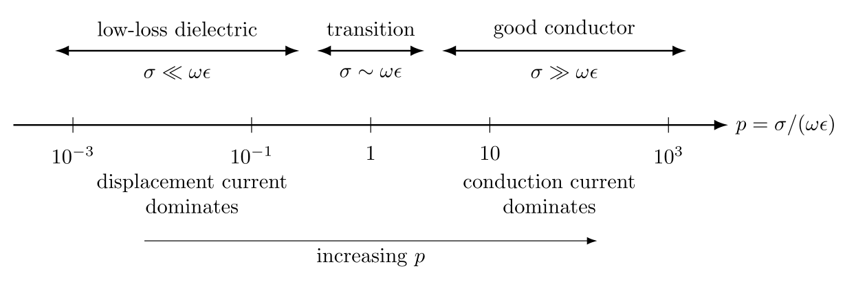
Figure 3. Material propagation regimes are organized by the ratio σ∕(ω𝜖). The same
material can move between regimes as frequency changes.
Because p contains ω in the denominator, increasing frequency tends to make a fixed material
appear more dielectric-like.
11 Low-loss dielectric approximation
For
use
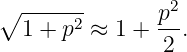
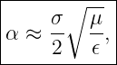
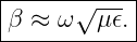
Then
and
Thus a weakly conducting dielectric has almost the same phase behavior as a lossless dielectric but
slowly loses amplitude.
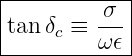
The ratio
may be interpreted as a conduction-loss tangent. Real dielectric loss can also be represented by a
complex, frequency-dependent permittivity, so the full loss tangent can contain more than this
ohmic contribution [3, 4].
12 Example: a slightly lossy dielectric
Take
Then
so the low-loss approximation is appropriate.
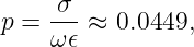
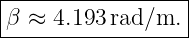
The exact formulas give
and
Therefore
and
After 10 m the field amplitude is reduced by
13 Attenuation in nepers and decibels
If
then
20 log 10 | = 20 log 10(e−αz) | (63)
|
| = −8.686 αz. | (64) |
Hence
Since power is proportional to field amplitude squared,
and therefore
The same numerical dB attenuation results whether one starts from field amplitude with 20 log 10
or power with 10 log 10.
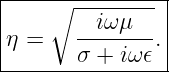
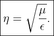
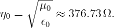
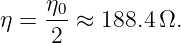
14 Intrinsic impedance of a material
For a uniform plane wave define
With the eiωt convention,
For a lossless dielectric,
In vacuum,
For 𝜖r = 4 and μr = 1,
This impedance is a field ratio, not a lumped resistor inserted in the path of the wave.
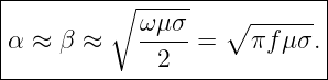
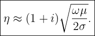
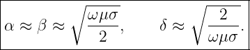
15 The good-conductor limit
For
the exact expressions simplify to
The intrinsic impedance becomes
The wave both accumulates phase and loses amplitude rapidly.
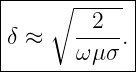
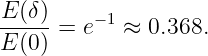
16 Skin depth
Define
For a good Conductor,
At one skin depth,
At two and three skin depths,
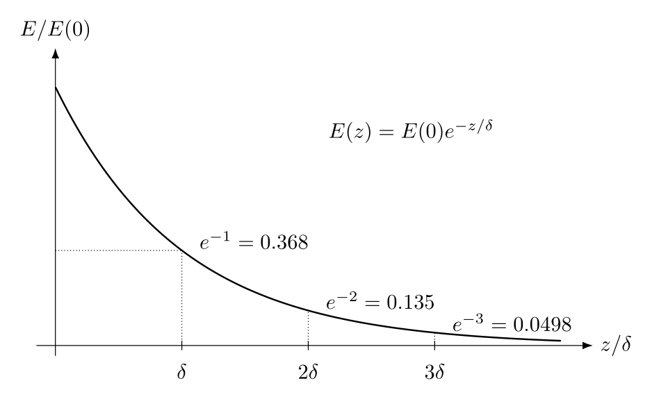
Figure 4. Skin depth is the distance over which field amplitude falls by the factor 1∕e.
17 Example: copper at 1 MHz
Take
The good-conductor approximation gives
so
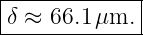
The field is strongly attenuated within a fraction of a millimeter. This is the electromagnetic basis
of the RF skin effect in good conductors.
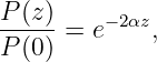
18 Power flow also decays
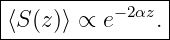
EM17 introduced the time-averaged Poynting vector. In a lossy medium,
so power density behaves as
The lost electromagnetic power is transferred to matter. For an ohmic conductor,
which is the local electromagnetic-to-thermal energy transfer appearing in Poynting’s
theorem.
19 Complex permittivity viewpoint
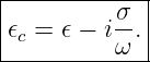
The conduction term can be absorbed algebraically into a complex permittivity:
Define
Then
This form is useful because real material polarization can itself introduce frequency-dependent
complex permittivity.
20 Dispersion: when phase speed depends on frequency
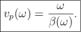
Real material parameters can depend on frequency:
Then
and
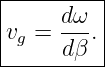
A pulse contains a range of frequencies. The speed of a narrowband envelope is described by the
group velocity
In a nondispersive medium, β ∝ ω and vg = vp. In a dispersive medium they need not be
equal.
21 What remains unchanged from the vacuum plane wave
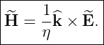
A uniform plane wave in a homogeneous isotropic medium remains transverse:
The fields are related by
In a lossless medium, η is real and E and H are in phase. In a lossy medium, η is complex, so they
generally have a phase offset.
Polarization from EM19 remains a transverse-vector property. An isotropic medium can change
phase velocity and amplitude without selecting a preferred transverse direction. Anisotropic
materials can do more and can alter the polarization state itself; that lies beyond the scope of this
introductory propagation article.
22 A compact hierarchy of propagation models
The same Maxwell equations underlie every regime. What changes is the relative importance of
displacement current, conduction current, and material response.
23 Connection to RF propagation
The propagation constant
is the compact bridge from Maxwell’s Equations to engineering propagation calculations. The
attenuation constant α determines loss through matter. The phase constant β determines
wavelength and phase delay. The intrinsic impedance η determines the electric-to-magnetic field
ratio.
The next natural question is what happens when a wave reaches a boundary between two different
media. That problem introduces impedance mismatch, reflection, transmission, refraction, and the
boundary conditions that connect the fields on the two sides.
24 Summary
For a homogeneous linear isotropic medium,
For time-harmonic propagation,
The corresponding plane wave is
The principal propagation quantities are
For a lossless dielectric,
For a good conductor,
These relations explain how the same electromagnetic wave can propagate nearly without loss
through one material, slow down and shorten its wavelength in another, or decay within
micrometers of the surface of a good conductor.
References
References
[1] D. J. Griffiths, Introduction to Electrodynamics, 4th ed., Cambridge University Press,
2017.
[2] J. D. Jackson, Classical Electrodynamics, 3rd ed., Wiley, 1999.
[3] D. K. Cheng, Field and Wave Electromagnetics, 2nd ed., Addison-Wesley, 1989.
[4] F. T. Ulaby and U. Ravaioli, Fundamentals of Applied Electromagnetics, 7th ed.,
Pearson, 2015.
[5] C. A. Balanis, Advanced Engineering Electromagnetics, 2nd ed., Wiley, 2012.



























![[α ] = Np/m, [β] = rad/m.](https://images.physicslibrary.org/cache/objects/1443/make4ht/ElectromagneticWavesAntennasAndRFWavePropagationInMaterials41x.png)




![|------------------------------|
| ∘ -μ𝜖[∘ ------ ]1∕2 |
|α = ω --- 1 + p2 − 1 ,|
----------2--------------------](https://images.physicslibrary.org/cache/objects/1443/make4ht/ElectromagneticWavesAntennasAndRFWavePropagationInMaterials46x.png)
![|------∘-----------------------|
| μ𝜖[∘ ------ ]1∕2 |
|β = ω --- 1 + p2 + 1 . |
----------2--------------------](https://images.physicslibrary.org/cache/objects/1443/make4ht/ElectromagneticWavesAntennasAndRFWavePropagationInMaterials47x.png)