FS19: Deriving the Complex Fourier Coefficients
The real Fourier series describes a periodic function by adding sine and cosine harmonics. FS18
showed that these are two parts of a more compact function-space direction: the complex
exponential einx. We now answer a very specific question: given a periodic function f, how much of
the mode eimx does it contain?
This is the same projection problem first studied in FS02. The calculation looks unfamiliar only
because the basis functions and coefficients may now be complex. We will derive the coefficient
directly from a finite expansion, carefully distinguish the selected harmonic m from the running
index n, and only then discuss an infinite series. The essential result on [−L,L] will
be
where m may be any integer, positive, negative, or zero.
The minus sign in the exponential, the factor 1∕(2L), and the presence of negative indices all
follow from the same orthogonal-projection argument. None needs to be memorized
independently.
1 Why replace two real functions with one complex function?
Euler’s formula, derived in FS18, states
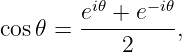
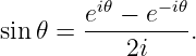
The two opposite complex rotations recover cosine and sine:
Hence a representation involving both cos(nx) and sin(nx) can be reorganized using modes einx for
integer n. The positive and negative indices record opposite senses of rotation in the complex
plane; they are not two unrelated kinds of physical oscillation.
For an interval of length 2L, define the complex Fourier basis functions
Each mode satisfies
and its spatial angular Wavenumber is nπ∕L. The allowed harmonics are integer-spaced because
the entire sum must repeat after 2L.
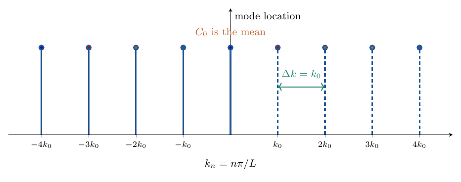
Figure 1. The complex basis contains negative, zero, and positive integer harmonics. Their
wavenumbers are equally spaced, with k0 = π∕L. The stems indicate mode locations, not specific
coefficient magnitudes.
2 The inner product must use complex conjugation
FS02 introduced, for real functions, the inner product ∫
f(x)g(x) dx. For complex functions we
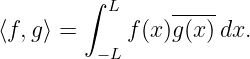
need the Hermitian inner product. In the convention used here it is
The overline means complex conjugation. This convention is linear in the first argument and
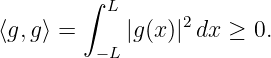
conjugate-linear in the second. In particular,
Without conjugation, ∫
g(x)g(x) dx can be zero or even complex for a nonzero complex function. It
therefore cannot generally serve as a squared length.
For the exponential basis,
Thus the negative sign in Equation (1) comes directly from the complex inner product: to measure
the component along ϕm, we multiply by its complex conjugate.
Derive complex exponential orthogonality
Calculate the inner product of two modes:
| ⟨ϕn,ϕm⟩ | = ∫
−LLeinπx∕Le−imπx∕L dx | |
|
| = ∫
−LLei(n−m)πx∕L dx. | (10) |
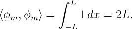
There are two different cases. First, if n = m, then the integrand is 1 everywhere, so
Second, when n≠m, set q = n − m. Because q is a nonzero integer,
| ∫
−LLeiqπx∕L dx | = 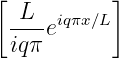 −LL | |
|
| =  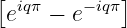 | |
|
| =   | |
|
| = 0. | (12) |
The result is
where the Kronecker delta is 1 if n = m and 0 otherwise.
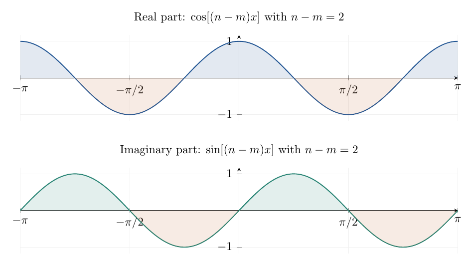
Figure 2. When n≠m, the real and imaginary parts of the product ei(n−m)x cancel over the full
symmetric period. When n = m, the product equals 1 and its integral is 2π.
3 Begin with a finite complex Fourier expansion
Suppose a function is exactly a finite combination of complex modes:
Here n is a running index: it visits every integer from −N to N. Each coefficient Cn is a fixed
complex number associated with the corresponding mode.
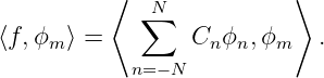
We want just one coefficient, Cm. Keep m fixed and take the inner product of both sides of
Equation (14) with ϕm:
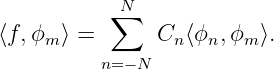
Use linearity in the first argument. Because the expansion is finite, no interchange of an infinite
sum and an integral is involved:
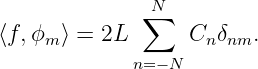
Substitute the orthogonality relation from Equation (13):
Every term with n≠m has δnm = 0. The one term with n = m has δmm = 1. Thus
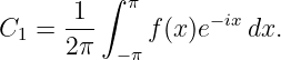
Solve for Cm:
This is the complex Fourier coefficient formula. The denominator is the squared norm ∥ϕm∥2 = 2L,
exactly as in FS02.
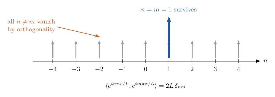
Figure 3. Taking the inner product against the selected mode m acts as an orthogonality filter.
Every running-index term n≠m vanishes; only the matching mode remains.
4 A five-term example makes the index filtering concrete
The summation notation hides a simple operation. Let L = π, let N = 2, and suppose
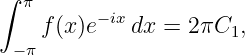
We want to isolate C1 without calculating any other coefficient. Multiply by e−ix and integrate
from −π to π:
| ∫
−ππf(x)e−ix dx = | C
−2 ∫
−ππe−3ix dx | |
|
| + C−1 ∫
−ππe−2ix dx | |
|
| + C0 ∫
−ππe−ix dx | |
|
| + C1 ∫
−ππ1 dx | |
|
| + C2 ∫
−ππeix dx. | (21) |
Every integral containing a nonzero integer multiple of x in the exponential is zero. Only the
fourth integral remains, and it equals 2π. Therefore
so
Observe the logic carefully: the test function e−ix is the conjugate of the selected mode eix. The
actual eix term becomes 1 under multiplication; every mismatched term remains a nonconstant
harmonic and integrates to zero.
5 From an exact finite sum to a general Fourier series
A general periodic function need not be a finite harmonic polynomial. We therefore define its
coefficients using the same projection integrals,
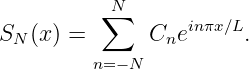
and form the partial sums
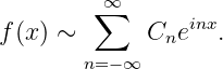
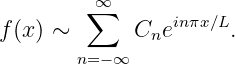
Formally, the complex Fourier series is
The symbol ∼ intentionally avoids claiming pointwise equality at every x. Under appropriate
hypotheses, these partial sums converge to f in the L2 sense, and stronger pointwise
conclusions require additional assumptions. A complete convergence analysis belongs to
FS14–FS16.
The finite derivation gave an exact reason for the coefficient formula without presupposing that an
infinite series could be integrated term by term. More generally, if f is square-integrable, SN is its
orthogonal projection onto the finite span of modes −N,…,N. The coefficient formula remains
meaningful whether or not a particular pointwise series converges.
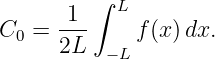
6 What does the zero-frequency coefficient mean?
Set n = 0 in Equation (24). Since e0 = 1,
For a real-valued function, this is its average over one period. It is the same DC component called
a0∕2 in the real Fourier-series convention.
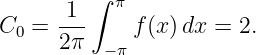
For example, if f(x) = 5 + 2 cos(3x) on [−π,π], then
The oscillating cosine contributes no average. Unlike the real-series formula a0 = π−1 ∫ f, the
complex coefficient C0 already is the constant term. There is no extra factor 1∕2 in the complex
expansion.
7 A complete finite-signal example
Consider the real periodic waveform
We will calculate its complex coefficients and reconstruct it exactly.
Step 1: coefficient at zero frequency
The average is
Step 2: coefficients at n = 1 and n = −1
From Equation (24),
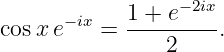
The constant and the sin 2x terms vanish by orthogonality. For the remaining term,
use
Consequently
The same calculation, or reality of f, gives C−1 = 3∕2.
Step 3: coefficients at n = 2 and n = −2
Now test against e−2ix. Only the sine term contributes. Using Equation (4),
Multiply this term by e−2ix:
It follows that
| C2 | =  ∫
−ππ  1 − e−4ix  dx | |
|
| = i. | (36) |
The opposite index gives C−2 = −i. Every Cn with |n| > 2 is zero.
Step 4: reconstruct the original signal
Substitute the five nonzero coefficients:
The first pair gives 3 cos x, while the second pair gives −2 sin 2x. We have recovered exactly the
original real waveform.
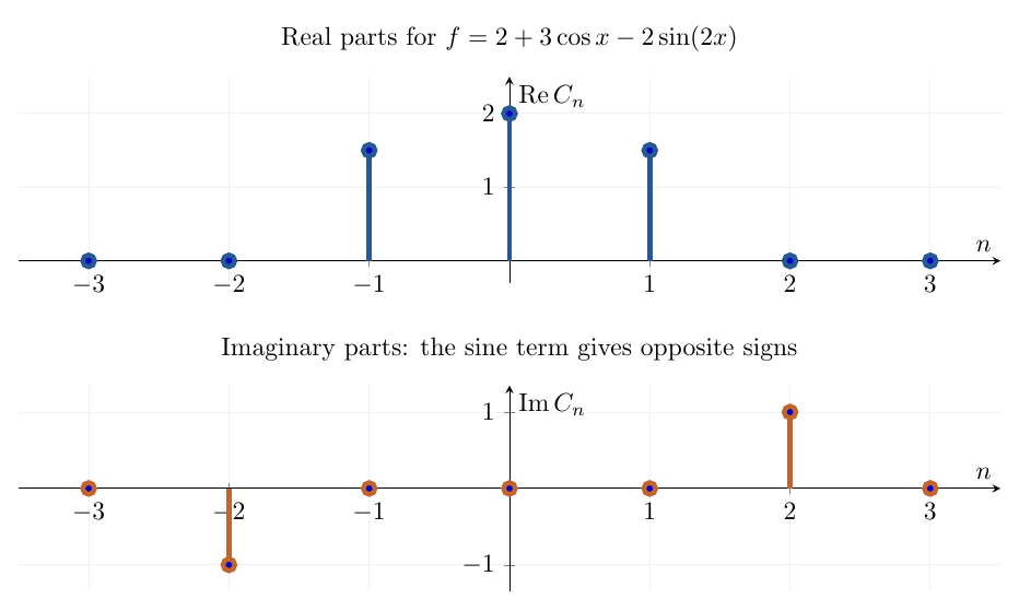
Figure 4. The finite-signal example has a real, nonzero DC coefficient, a real symmetric pair C±1,
and a purely imaginary pair C±2 of opposite signs.
8 Why real signals have conjugate-symmetric coefficients
If f(x) is real-valued, then f(x) = f(x). Start from
Taking the complex conjugate, with conjugation passed inside the integral, gives
| Cn | =  ∫
−LLf(x)e−inπx∕L dx | |
|
| =  ∫
−LLf(x)einπx∕L dx | |
|
| = C−n. | (39) |
Therefore
This is a fundamental consistency check. A real waveform does not require its complex coefficients
to be real. It requires the negative-frequency coefficient to be the complex conjugate of its
positive-frequency partner. As a result, their sum is real:
For example, if C2 = 1 − 3i, then C−2 = 1 + 3i. An arbitrary complex-valued signal need not obey
this symmetry.
9 Worked waveform: the odd square wave
Return to the FS07 odd square wave of amplitude A:
Its average is zero, so C0 = 0. For nonzero integer n, calculate directly:
| Cn | =  ∫
−ππf(x)e−inx dx | |
|
| =  ∫
−ππf(x)  cos(nx) − i sin(nx) ![]](https://images.physicslibrary.org/cache/objects/1579/make4ht/DerivingTheComplexFourierCoefficients54x.png) dx. | (43) |
Because f is odd and cos(nx) is even, f(x) cos(nx) is odd and integrates to zero. Because
f(x) sin(nx) is even, its integral is twice its positive-half integral:
| Cn | = − ∫
0πA sin(nx) dx | |
|
| = −  1 − (−1)n ![]](https://images.physicslibrary.org/cache/objects/1579/make4ht/DerivingTheComplexFourierCoefficients58x.png) . | (44) |
Thus
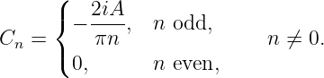
The nonzero coefficients are purely imaginary. They satisfy C−n = Cn, because reversing
n reverses the sign of the imaginary value. The real sine-series harmonics from FS07
reappear when each positive-frequency term is combined with its negative-frequency
partner.
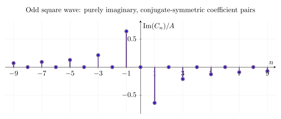
Figure 5. The imaginary parts of the odd square wave’s complex coefficients. Positive and negative
odd-harmonic coefficients have opposite signs, while every even-harmonic coefficient vanishes.
The values assigned to a square wave precisely at its jumps do not change these coefficients:
altering a function at finitely many points leaves all the coefficient integrals unchanged.
10 Worked waveform: centered rectangular pulse
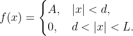
Consider a period-2L waveform with amplitude A and half-width d, where 0 < d < L:
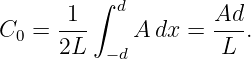
The waveform is even. Its zero-frequency coefficient is the mean,
For n≠0,
| Cn | =  ∫
−dde−inπx∕L dx | |
|
| =  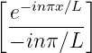 −dd | |
|
| =  sin  . | (48) |
Every Cn is real, and C−n = Cn. This matches the fact that the waveform is even. The magnitude
envelope is sinc-like; harmonics can also have alternating signs.
In time coordinates, define the pulse duration τ = 2d and the period T = 2L mathematically after
replacing spatial x by time t. The duty cycle becomes D = τ∕T = d∕L, and the coefficients can be
written
with sinc(z) = sin z∕z and sinc(0) = 1. This form includes C0 = AD by continuity. It is the discrete
line spectrum of a periodic pulse train, not the continuous Fourier transform of one isolated
pulse.
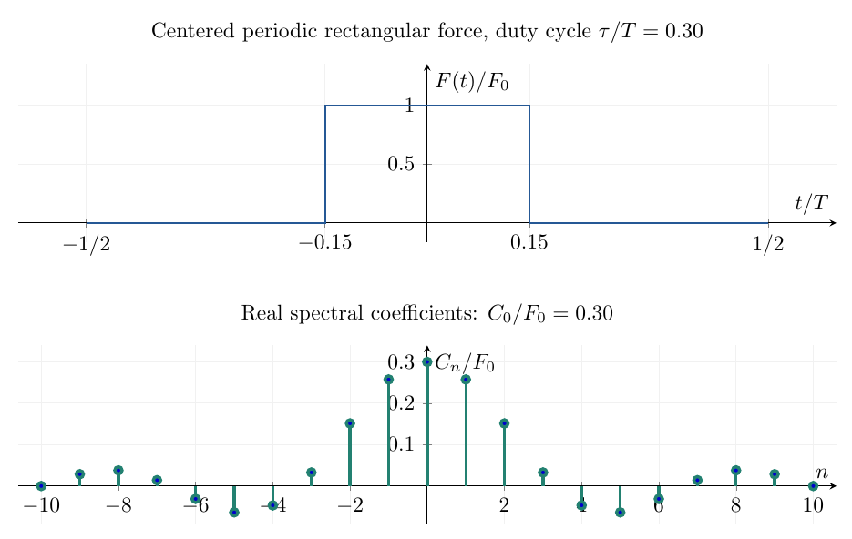
Figure 6. A centered periodic pulse with duty cycle 0.30 and its complex Fourier coefficients. Even
symmetry makes every coefficient real; the DC coefficient is the pulse’s duty-cycle-weighted mean.
11 Time-domain convention and frequency units
For a time-periodic signal with period T, let the fundamental angular frequency be
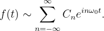
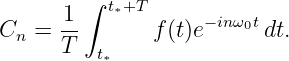
The corresponding complex basis is einω0t. With an arbitrary period starting at t
∗, the time-domain
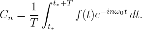
coefficient is
For a periodic integrable signal, the value is independent of the chosen whole-period interval. For a
centered interval one may choose t∗ = −T∕2.
The inverse series has the same e+inω0t sign convention used in the finite derivation:
Do not mix this angular-frequency convention with the hertz convention f0 = 1∕T.
Since ω0 = 2πf0, one may equivalently write ei2πnf0t. The normalizing factor remains
1∕T.
Dimensional analysis gives a useful check. If f is measured in volts, force, or displacement, then Cn
has the same units as f, because the integral contributes a factor of time that 1∕T removes. This
differs from the continuous Fourier transform, whose units include an additional factor of
time.
12 Time shifting changes coefficient phase
Let f(t) have coefficients Cn, and delay the waveform by t0:
Its coefficient is
Set u = t − t0, so t = u + t0 and dt = du. Periodicity allows the shifted integral to be moved back
to any whole period:
| Gn | =  ∫
t∗−t0t∗+T−t0
f(u)e−inω0(u+t0) du | |
|
| = e−inω0t0
 ∫
t∗−t0t∗+T−t0
f(u)e−inω0u du | |
|
| = Cne−inω0t0
. | (55) |
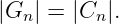
Because the multiplier has unit magnitude,
A pure time shift leaves harmonic magnitudes unchanged and rotates coefficient phases by
−nω0t0. The higher the harmonic index, the larger the phase rotation for the same
delay.
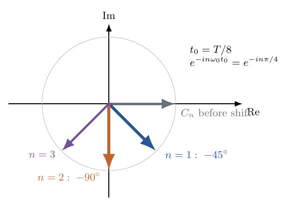
Figure 7. A delay t0 = T∕8 multiplies the nth coefficient by e−inπ∕4. The coefficient magnitude
stays fixed while the complex-plane phase rotates by an amount proportional to n.
13 Physical application: periodic force driving an oscillator
Consider a damped mass-spring system driven by a periodic force,
where M is mass, b is viscous damping, and k is stiffness. Suppose that F(t) is a centered
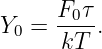
rectangular pulse train with force amplitude F0, pulse duration τ, and repetition period T. From
Equation (49), its complex force coefficients are
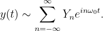
To find the periodic steady-state response, assume a mode-by-mode expansion
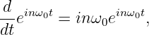
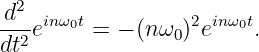
For a single mode, differentiation multiplies by inω0:
Insert the expansions into Equation (57) and equate coefficients of the same harmonic.
Orthogonality allows each mode to be handled independently:
Thus
This is the frequency-domain solution: every driving-force harmonic is multiplied by the oscillator’s
complex frequency response. For a damped system, these coefficients describe the periodic steady
state after the homogeneous transient has decayed.
At n = 0, inertia and damping contribute nothing. The static response is
If a harmonic lies near nω0 ≈ , the system can amplify that component relative to
neighboring harmonics, provided damping is not too large. The resonance behavior is set by the
denominator, not just by the pulse’s input spectrum.
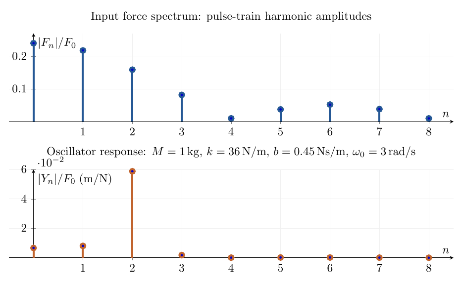
Figure 8. An illustrative pulse-train force and the resulting oscillator displacement spectrum for
the parameter values shown. The harmonic closest to the natural frequency can dominate the
response even when it is not the largest input-force harmonic.
This example illustrates why complex coefficients are more than a convenient notation. Their
magnitudes represent mode strengths, and their phases preserve the time alignment needed when
reconstructing the physical displacement.
14 How complex coefficients relate to the real coefficients
There is only one underlying periodic function. The real and complex series are two
coordinate systems for describing it. For the standard period-2π convention, one may
write
and also
Substitute Equations (3) and (4) into one harmonic pair:
| an cos(nx) + bn sin(nx) | =  einx | |
|
| +  e−inx. | (67) |
The coefficient identification is
Conversely,
FS20 will develop these relationships more systematically, including a careful comparison of
amplitudes, phases, and symmetric spectral plots. For now, the main lesson is that a real sinusoid
generally requires two conjugate complex-frequency terms.
15 Another connection to FS12: finite projection energy
For a finite complex approximation SN, orthogonality also gives a squared-norm identity:
| ∥SN∥2 | = ⟨S
N,SN⟩ | |
|
| = ∑
n=−NN ∑
m=−NNC
nCm⟨ϕn,ϕm⟩ | |
|
| = 2L∑
n=−NN|C
n|2. | (70) |
This equation is exact for every finite partial sum. Further, since SN is the orthogonal
projection of f onto the retained mode space, the residual rN = f − SN is orthogonal to SN.
Therefore
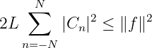
The resulting inequality
is the finite form of Bessel’s inequality. Passing to an equality for the full infinite basis requires the
completeness and convergence theory of Parseval’s theorem, developed in FS13. No infinite-energy
identity is presumed here.
16 Subtle points and common mistakes
Mixing two different inner-product conventions
Our convention is ⟨f,g⟩ = ∫
fg, linear in the first argument. Many textbooks use ∫
fg, linear in
the second argument. Both are valid, but one must use a consistent convention when
deriving projection coefficients. Equation (19) is consistent with the convention stated in
Equation (7).
Omitting the negative-frequency modes
The complex basis is indexed by all integers, not only positive indices. A real cosine needs both +n
and −n contributions. Omitting one generally produces a complex rotating phasor, not the
intended real waveform.
Confusing C0 with a0
In real Fourier notation the constant term is a0∕2. In complex Fourier notation it is already C0.
The common normalization conventions are consistent when C0 = a0∕2.
Assuming every periodic function is smooth
A waveform with jumps still has perfectly well-defined coefficient integrals if it is integrable.
Convergence precisely at the jump is a separate question. The complex basis does not
remove Gibbs oscillations or pointwise-convergence issues; it reorganizes the same Fourier
information.
Confusing complex Fourier series with the Fourier transform
For a periodic signal, the coefficients Cn correspond to discrete harmonic frequencies nω0. In
FS26, an isolated nonperiodic pulse is described by a continuous transform F(ω). In the
periodic-repetition construction for an isolated integrable pulse, Cn = F(ωn)∕T. This is a
special bridge between the two descriptions, not an equality of their units or general
definitions.
17 Short self-checks with answers
- If f(x) = 7 on [−π,π], what are its complex coefficients? Answer: C0 = 7 and Cn = 0
for every n≠0.
- For a real signal, if C3 = 2 − 5i, what is C−3? Answer: 2 + 5i.
- If f(x) = 4 cos(2x), identify its nonzero coefficients. Answer: C2 = C−2 = 2.
- If f(x) = 6 sin x, what are C1 and C−1? Answer: C1 = −3i and C−1 = 3i.
- What is the coefficient normalization on an interval [−3, 3]? Answer: 1∕(2L) = 1∕6,
using e−inπx∕3 in the integrand.
- If a periodic voltage is shifted by T∕4, what happens to C2? Answer: it is multiplied
by e−i2π∕2 = −1; its magnitude is unchanged.
18 What FS19 has established
We started from FS18’s complex exponential basis and used the FS02 projection principle without
shortcuts. Conjugation determined the sign of the extracting exponential. Orthogonality
removed all unwanted harmonics. The mode norm supplied the factor 2L. The outcome
was
with the period-T equivalent
We then used these formulas for finite harmonics, a square wave, a pulse train, and a
mechanical oscillator. These examples establish why complex Fourier coefficients are
useful mathematical coordinates and physically meaningful spectral amplitudes and
phases.
The natural next step, FS20, is to put the real and complex descriptions side by side until the
conversion between an,bn and Cn becomes automatic.
References
[1] E. Kreyszig, Advanced Engineering Mathematics, 10th ed., Wiley, 2011, chapters on
Fourier analysis.
[2] A. V. Oppenheim, A. S. Willsky, and S. H. Nawab, Signals and Systems, 2nd ed.,
Prentice Hall, 1997, chapters on Fourier series.
[3] R. N. Bracewell, The Fourier Transform and Its Applications, 3rd ed., McGraw-Hill,
2000.
[4] PhysicsLibrary, FS02, FS06, FS11, FS12, and FS18 prerequisite lectures.

















 =