Calculus of Variations: Strong Extrema and Sufficiency Conditions
The Euler–Lagrange equation tells us which admissible curves are stationary. CV11 and CV12 then
used the second variation, the Legendre condition, and the Jacobi equation to determine when a
stationary curve behaves locally like a minimum with respect to sufficiently small changes in both
the curve and its slope.
A final difficulty remains. A curve can be extremely close to an extremal in position while having a
very different derivative. Such competitors are invisible to a purely C1-local test, yet they matter
for a strong minimum. The classical tool that detects them is the Weierstrass excess function,
usually called the Weierstrass E-function.
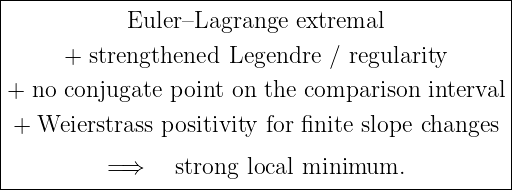
The conceptual progression is
Classical sufficiency theory is developed in different but equivalent forms in Bolza, Bliss, Gelfand
and Fomin, Weinstock, Sagan, and van Brunt [6, 5, 1, 4, 3, 2].
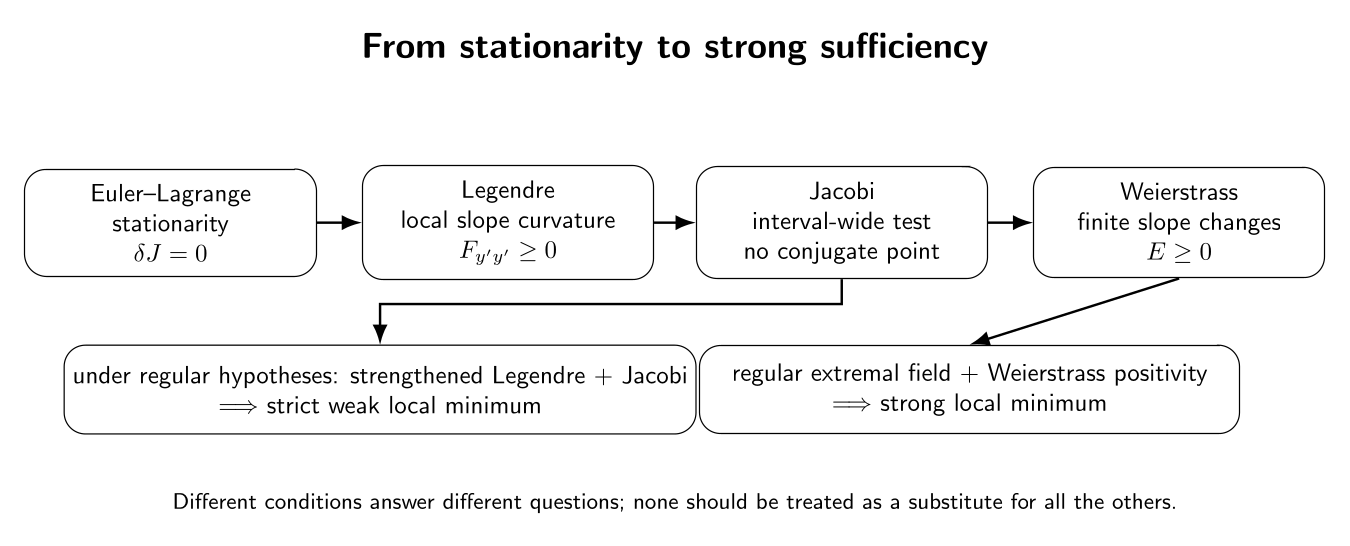
Figure. The major conditions answer different questions. Euler–Lagrange detects
stationarity; Legendre and Jacobi control infinitesimal slope changes over an interval; the
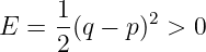
Weierstrass condition controls finite changes of slope required for strong extrema.
1 Learning objectives
After completing this entry, the reader should be able to:
- distinguish weak and strong local minima using C1 and C0 neighborhoods;
- explain why a strong minimum must tolerate competitors whose slopes differ greatly
from the extremal slope;
- derive and interpret the Weierstrass excess function;
- prove that the Weierstrass condition implies the Legendre condition in the infinitesimal
limit;
- construct a stationary curve that is a weak minimum but not a strong minimum;
- explain why the Weierstrass condition alone is not sufficient;
- define a field of extremals and the associated slope field;
- derive the Hilbert invariant integral and its exactness condition;
- prove a classical strong-minimum sufficiency theorem using the Hilbert integral and
the excess function;
- connect the no-conjugate-point condition with the local construction of a field of
extremals;
- recognize special convexity structures that give global rather than merely local
conclusions.
2 Weak and strong extrema revisited
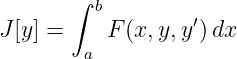
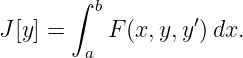
Let
on an admissible class of piecewise C1 curves satisfying fixed endpoint conditions.
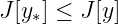
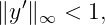
A weak local minimum y∗ is a curve for which there exists ρ > 0 such that
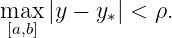
whenever the competitor satisfies a C1-type closeness requirement such as
A strong local minimum requires the same inequality for every admissible competitor that is
sufficiently close only in position:
The derivative of the competitor need not be close to y∗′. Therefore
but the converse can fail.
2.1 Why strong closeness is more demanding
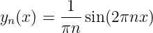
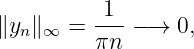
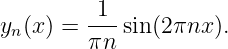
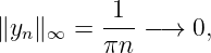
A high-frequency perturbation can have tiny amplitude but a large derivative. For example,
on [0, 1] satisfies
while
has derivative amplitude 2 for every n.
Thus yn approaches the zero function strongly in the C0 sense but not weakly in the C1 sense used
here.
3 The Weierstrass excess function
Fix x and y. Let
be the slope of a candidate extremal and let
be a competing slope. The tangent line to the function F(x,y,⋅) at p is
The vertical difference between the true value at q and this tangent approximation
is
This is the Weierstrass excess function.
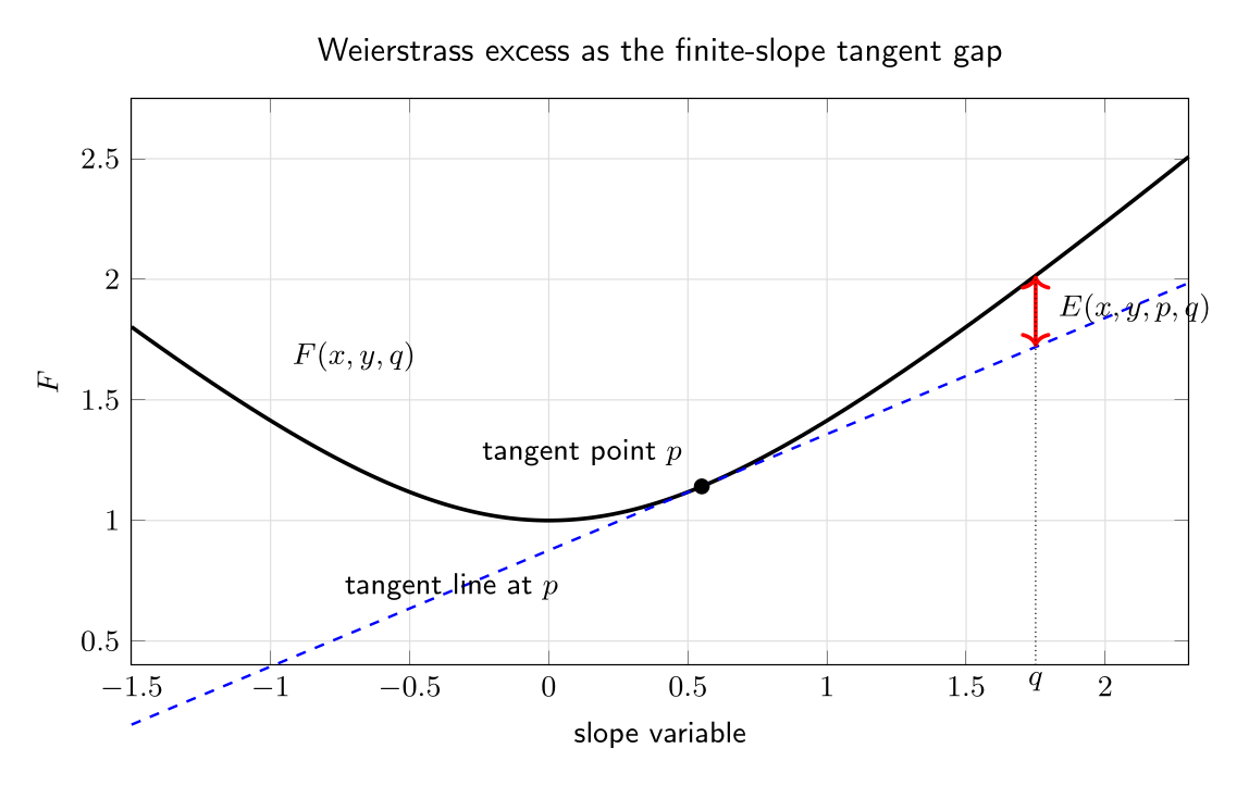
Figure. At fixed (x,y), the Weierstrass excess is the vertical gap between F at a finite
comparison slope q and the tangent line to F at the extremal slope p. It therefore probes
finite slope changes rather than only infinitesimal ones.
The basic geometric interpretation is
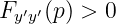
If F is convex as a function of its slope argument, then
for every p and q. Strict convexity gives strict positivity whenever q≠p.
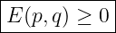
4 The Weierstrass necessary condition
A classical necessary condition for a strong local minimum is the following.
Weierstrass necessary condition
Suppose F is sufficiently smooth and y∗ is a strong local minimizer. Then along the
extremal,
for every interior point x and every finite comparison slope q for which the local comparison is
admissible.
The important phrase is every finite comparison slope. The Legendre condition checks only what
happens when q is infinitesimally close to p.
4.1 Why a finite-slope test appears
A strong neighborhood constrains the vertical displacement of the competitor but not its slope.
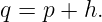
Over a very short interval of length h, one may therefore replace the extremal slope
p by a finite slope q while keeping the resulting vertical displacement only of order
h.
A short reconnecting segment restores the competitor to the original curve. When the variation is
shrunk around a fixed interior point, the leading-order change in the functional is proportional
to
If this number were negative, the small broken-line competitor could be made arbitrarily close in
C0 while lowering J. That would contradict strong minimality. This is the geometric core of
Weierstrass’s argument [6, 5, 2].
5 Legendre is the infinitesimal limit of Weierstrass
Set
Taylor expansion in the slope argument gives
Substituting into the definition of E gives
Therefore, if
for all sufficiently small positive and negative h, then
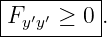
So the Legendre condition is the local quadratic shadow of the Weierstrass condition.
The converse is false. Knowing only
says that the tangent line is locally supporting near p; it does not guarantee that F(q) remains
above that tangent line for slopes far away from p.
6 A curve that is weakly minimizing but not strongly minimizing
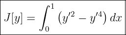
Consider
with fixed endpoints
The zero function
is stationary because F depends only on y′ and
vanishes along y∗′ = 0.
6.1 Weak local minimality
If a competitor is sufficiently close in C1 so that
then
Hence
Equality with the fixed endpoints occurs only when y′≡ 0, hence only when y ≡ 0. Thus y∗ is a
strict weak local minimum.
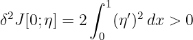
Its second variation is also positive:
for every nonzero fixed-endpoint variation.
6.2 Failure of strong minimality
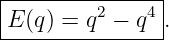
For the extremal slope p = 0, the Weierstrass function is
This becomes negative whenever
Now use the small-amplitude, high-frequency competitors
They satisfy the endpoint conditions and
but
Therefore
| J[yn] | = ∫
01 dx | (37)
|
| = 4 − 16  | (38)
|
| = 2 − 6 | (39)
|
| = −4 . | (40) |
Thus arbitrarily C0-close competitors have smaller functional value:
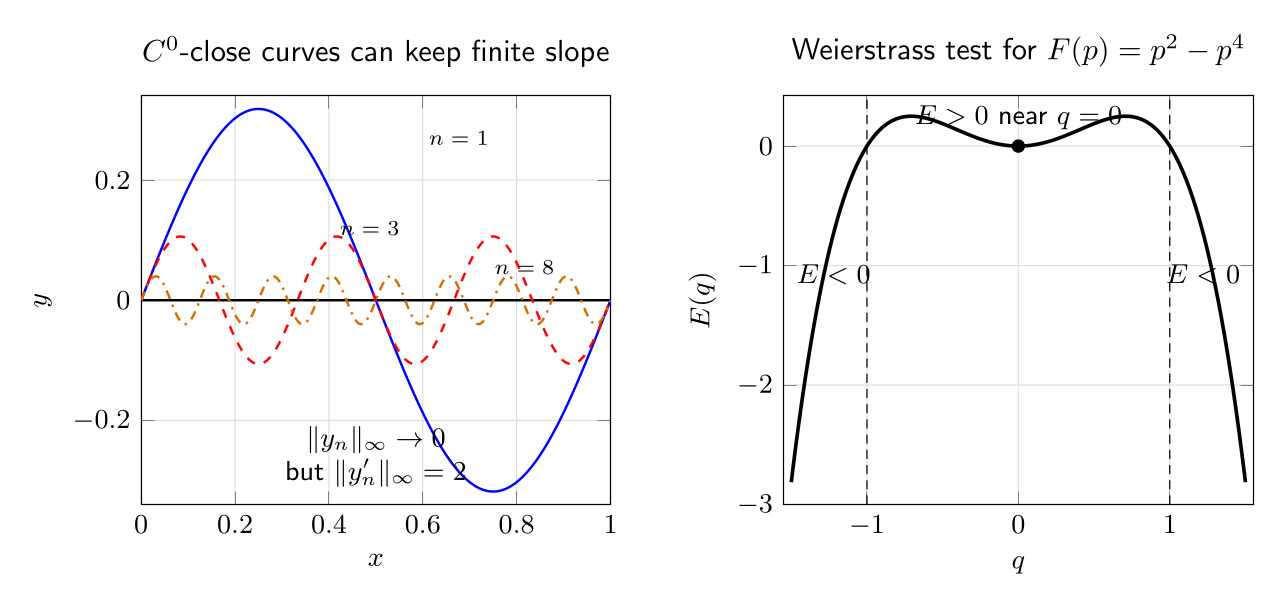
Figure. The left panel shows how high-frequency competitors can remain close in position
while retaining finite slope. The right panel shows the same failure through the Weierstrass
excess: E(q) is positive near q = 0 but negative for sufficiently large slope changes.
This example is one of the most useful conceptual separations in the subject:
7 The strengthened Weierstrass condition
For sufficiency arguments one usually imposes a strict version:
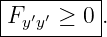
This is called a strengthened Weierstrass condition.
It is stronger than the necessary condition E ≥ 0. It provides strict separation from the tangent
line for every competing slope.
If F is strictly convex in y′, then the strengthened Weierstrass condition holds automatically at
every slope.
However, this still does not by itself prove that a stationary curve is minimizing. The y-dependence
of the functional and the geometry of neighboring extremals still matter.
8 Why Weierstrass alone is not sufficient
Consider the harmonic-oscillator action on [0,T],
The zero curve is stationary. For any baseline slope p and comparison slope q,
whenever q≠p.
So the strengthened Weierstrass condition holds globally in the slope variable.
Nevertheless, CV12 showed that the first conjugate point occurs at
For
there are directions with negative second variation, and the zero solution is not a minimum.
Therefore
The Jacobi condition supplies the missing interval information.
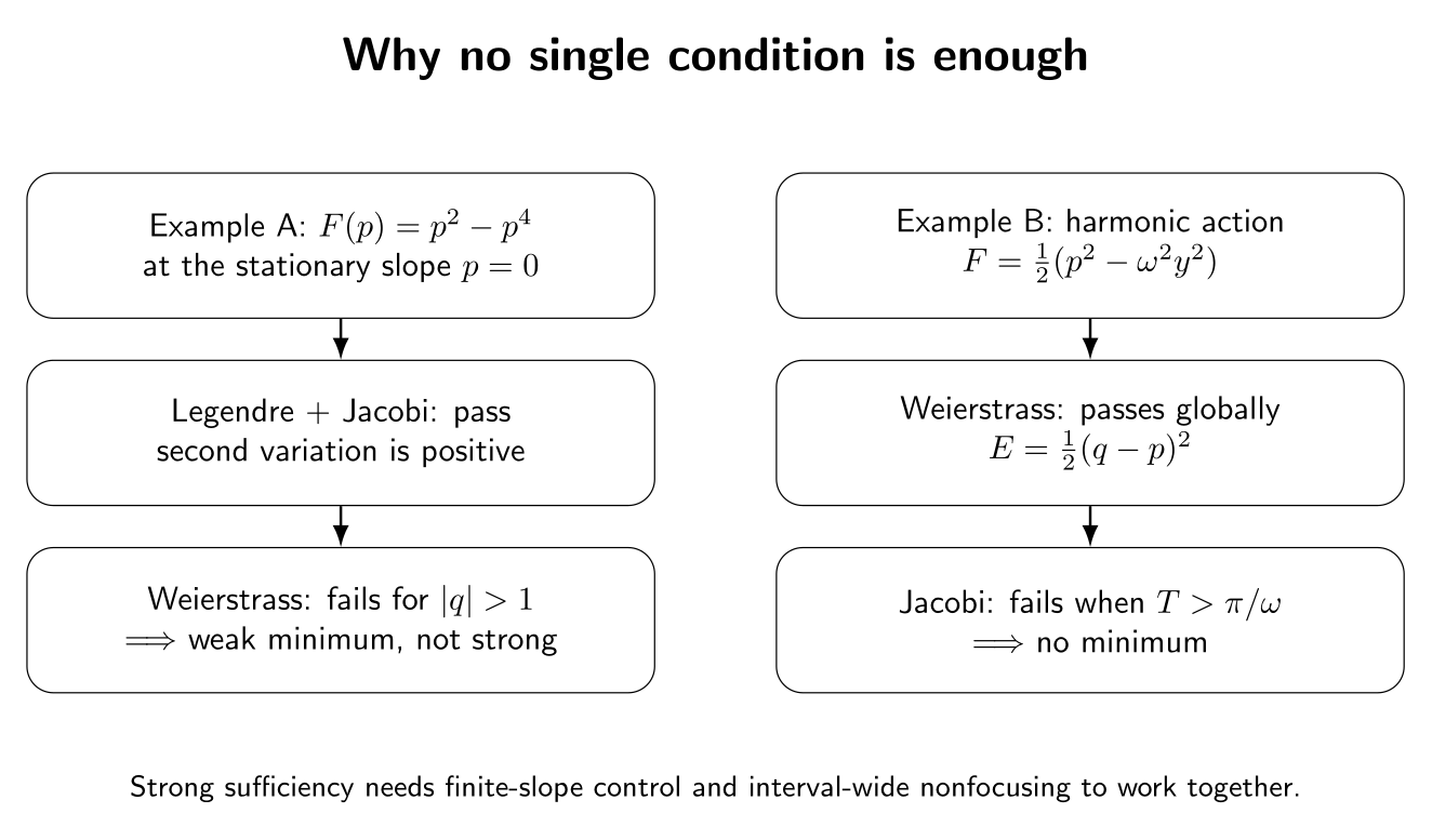
Figure. Two independent failure modes explain why strong sufficiency requires more than
one condition. Legendre–Jacobi theory can succeed while Weierstrass fails, giving only a
weak minimum; or Weierstrass can succeed while Jacobi fails, giving no minimum at all.
9 Fields of extremals
The classical strong-sufficiency proof uses a neighborhood filled by neighboring extremals.
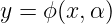
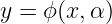
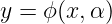
A field of extremals is a one-parameter family
such that each curve obtained by holding α fixed satisfies the Euler–Lagrange equation, and the
family locally fills a region without folding onto itself.
If the relation
can be inverted locally for
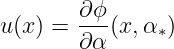
then the slope of the field extremal passing through (x,y) is
Thus the field converts a family of extremals into a slope field P(x,y).
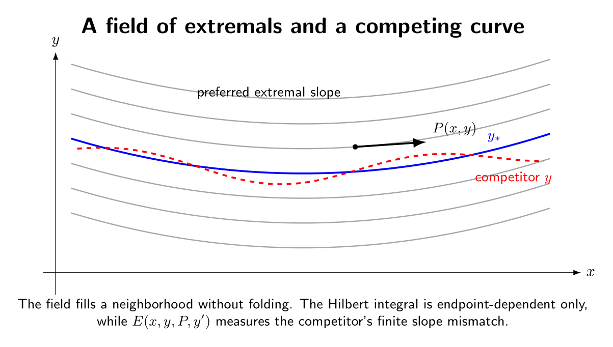
Figure. A regular field of extremals assigns a preferred extremal slope P(x,y) throughout
a neighborhood. A competing curve may cut across this field and may have slopes far from
P; the Weierstrass excess measures the local cost of that mismatch.
10 The Hilbert invariant integral
The field of extremals leads to a remarkable exact differential form.
Define
and
Now consider the one-form
10.1 Why the one-form is closed
Differentiate N with respect to x while holding y fixed:
Differentiate M with respect to y while holding x fixed:
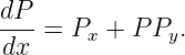
Along a field extremal, y′ = P and
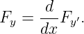
The Euler–Lagrange equation for every member of the field is
Expanding the total derivative gives
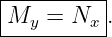
Substitute this into My:
| My | = Fy′x + PFy′y + Fy′y′Px + PFy′y′Py − PFy′y − PFy′y′Py | (61)
|
| = Fy′x + Fy′y′Px | (62)
|
| = Nx. | (63) |
Therefore
On a simply connected local field region, the one-form ω is exact. Hence its integral depends only
on the endpoints.
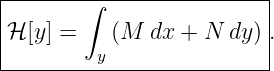
Define the Hilbert invariant integral
For two nearby curves with the same endpoints,
11 The key identity behind strong sufficiency
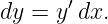
Along any competitor y(x) inside the field region,
Therefore
| ℋ[y] | = ∫
ab dx | (68)
|
| = ∫
ab dx. | (69) |
By the definition of the Weierstrass excess,
Hence
For the distinguished field extremal y∗,
so
and therefore
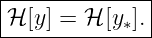
Since the Hilbert integral is endpoint dependent only,
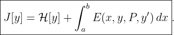
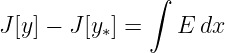
for every nearby competitor with the same endpoints. Subtracting gives the decisive
identity
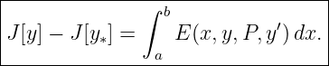
This formula is one of the cleanest sufficiency statements in the classical theory.
12 A classical strong-minimum sufficiency theorem
One standard formulation is the following [6, 5, 1, 2].
Strong sufficiency theorem, field form
Let y∗ be a fixed-endpoint extremal for
Assume there exists a regular field of extremals containing y∗ in a neighborhood 𝒰 of its graph,
and suppose
for every (x,y) ∈𝒰 and every admissible finite slope q.
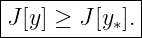
Then every admissible comparison curve lying in 𝒰 and having the same endpoints
satisfies
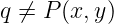
If the excess is strictly positive whenever
and the local field extremal joining the fixed endpoints is unique, then y∗ is a strict strong local
minimum.
12.1 Proof
The Hilbert-integral identity gives
If E ≥ 0 pointwise, then the integral is nonnegative. If E > 0 whenever the competitor slope differs
from the field slope, equality can hold only if the competitor follows the same extremal field line
almost everywhere. Local uniqueness then forces
Thus the conclusion is strong because no smallness assumption is imposed on y′− y∗′; only the
curve itself must remain inside the field neighborhood.
13 Where Jacobi enters the sufficiency theorem
The field-form theorem assumes that a regular field of extremals already exists. CV12 explains how
the Jacobi equation enters when one tries to construct such a field.
Consider a one-parameter family
of neighboring extremals. The derivative
is a Jacobi field.
If u vanishes again after the initial point, neighboring extremals refocus. At such a conjugate point
the local family fails to remain one-to-one. In contrast, the absence of a conjugate point prevents
this first-order focusing and is precisely the nondegeneracy needed in the classical construction of a
local extremal field.
Thus, under the standard regularity hypotheses, the practical sufficiency chain is
Different textbooks package the hypotheses somewhat differently; some state existence of an
extremal field directly, while others derive it from Jacobi-type assumptions [5, 6, 2].
14 Example: Dirichlet energy
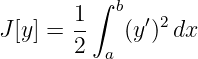
Consider
with fixed endpoints. The Euler–Lagrange equation is
so the extremal is the straight line
For
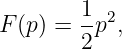
the excess function is
| E(p,q) | =  q2 −  p2 − (q − p)p | (90)
|
| =  (q − p)2 . | (91) |
Thus the strengthened Weierstrass condition holds globally.
In fact one can prove more directly that the straight line is the unique global minimizer.
Write
Then
| J[y] − J[y∗] | =  ∫
ab  dx | (93)
|
| = ∫
abmh′dx +  ∫
ab(h′)2 dx | (94)
|
| =  ∫
ab(h′)2 dx | (95)
|
| ≥ 0. | (96) |
Equality requires h′≡ 0 and the endpoints then give h ≡ 0.
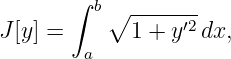
15 Example: planar arc length
For
let the straight-line extremal have constant slope p. Then
| E(p,q) | =  −  − (q − p)  | (98)
|
| = 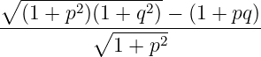 . | (99) |
By the Cauchy–Schwarz inequality,
so
with equality only when q = p.
This reproduces the strong local result. Convexity actually permits a global proof: the graph of
F(q) =  lies above its tangent at p, and the integrated tangent term vanishes because the
endpoints determine the average slope.
Thus the straight line is the unique shortest graph joining the two fixed endpoints.
16 A hierarchy of conclusions
The major conditions should not be treated as interchangeable.
|
|
|
| Question | Typical tool | What it controls |
|
|
|
| Stationary? | Euler–Lagrange | first variation |
|
|
|
| Infinitesimal slope curvature? | Legendre | local slope convexity |
|
|
|
| Interval-wide second-order sign? | Jacobi | conjugate points / focusing |
|
|
|
| Finite slope changes? | Weierstrass E | strong variations |
|
|
|
| Strong sufficiency? | extremal field + E ≥ 0 | C0-near competitors |
|
|
|
| Global minimum? | global convexity / exact identity | entire admissible class |
|
|
|
A useful memory aid is
17 Necessary versus sufficient conditions
The logical distinctions are essential.
17.1 Necessary conditions for a strong minimum
Under the usual regularity assumptions, a strong minimum must satisfy conditions such
as:
- Euler–Lagrange stationarity;
- the Legendre condition;
- the Jacobi no-interior-conjugate-point requirement in the regular case;
- the Weierstrass condition E ≥ 0.
Failure of any applicable necessary condition rules out strong minimality.
17.2 Sufficiency needs the conditions to work together
None of the pointwise conditions alone is enough.
- Positive second variation can still fail to control large slope changes, as the y′2 − y′4
example shows.
- Weierstrass positivity can hold while the Jacobi condition fails, as the long-interval
harmonic oscillator shows.
- Euler–Lagrange alone merely says the first variation vanishes.
The field-of-extremals theorem combines these ideas into an actual comparison formula for nearby
curves.
18 Common misconceptions
Misconception 1: “If Fy′y′ > 0, the extremal is a strong minimum.”
No. This condition controls only infinitesimal slope changes. The Weierstrass excess can become
negative for finite changes of slope.
Misconception 2: “A positive second variation proves strong minimality.”
Not in general. The second variation is a small-C1 statement. Strong competitors may be C0-close
while having large derivatives.
Misconception 3: “If E > 0, we no longer need Jacobi.”
No. The harmonic-oscillator example has strictly positive excess in slope but ceases to minimize
after the first conjugate point.
Misconception 4: “Strong means the perturbation is smaller.”
The terminology refers to the strength of the minimum property, not to a stronger norm. A
strong minimum survives a larger family of competitors because only C0 closeness is
required.
Misconception 5: “The Hilbert integral is an extra physical conservation law.”
Not generally. Here it is an exact line integral constructed from a field of extremals. Its endpoint
invariance is a mathematical comparison device.
19 Practical classification workflow
For a first-order fixed-endpoint problem, a useful procedure is:
- Derive the Euler–Lagrange equation and identify a stationary candidate y∗.
- Compute
- Form the second variation and apply the Jacobi test if interval-wide positivity is not
obvious.
- If only a weak local minimum is required, strengthened Legendre plus the Jacobi
condition may already provide the needed local sufficiency result under the standard
hypotheses.
- If a strong minimum is required, compute
- Test finite slope changes, not only q ≈ p.
- Establish or invoke a regular field of extremals around the candidate.
- Use the Hilbert-integral identity
for nearby competitors in the field.
- If a global result is desired, look for global convexity, completion-of-squares identities,
geometric inequalities, or other arguments that compare against the whole admissible
class.
20 What CV14 adds
CV13 completes the core local-extremum theory for first-order scalar functionals:
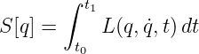
CV14 turns this machinery toward Classical Mechanics. Hamilton’s principle will identify the
action functional
and derive Lagrange’s equations for mechanical systems. The distinction between stationary action
and minimum action will be especially important: mechanical trajectories are stationary, but they
need not minimize the action over arbitrary time intervals.
Summary
Weak and strong extrema differ because strong comparison curves need only be close in position.
Their slopes may differ greatly from the extremal slope.
The Weierstrass excess function
measures the cost of a finite slope change relative to the tangent approximation at the extremal
slope.
For a strong minimum, the Weierstrass necessary condition requires
Its infinitesimal limit gives the Legendre condition
A regular field of extremals with slope field P(x,y) generates the Hilbert invariant integral and the
identity
This turns pointwise Weierstrass positivity into a strong local comparison theorem. The Jacobi
condition remains essential because it controls the interval-wide focusing of neighboring extremals
and supports the construction of a regular extremal field.
Thus the classical sufficiency picture is not one condition but a coordinated hierarchy:
under the corresponding regularity and field hypotheses.
References
[1] I. M. Gelfand and S. V. Fomin, Calculus of Variations, Dover Publications, 2000.
[2] Bruce van Brunt, The Calculus of Variations, Springer, 2004.
[3] Hans Sagan, Introduction to the Calculus of Variations, Dover Publications, 1992.
[4] Robert Weinstock, Calculus of Variations with Applications to Physics and
Engineering, Dover Publications, 1974.
[5] Gilbert Ames Bliss, Lectures on the Calculus of Variations, University of Chicago
Press, 1946.
[6] Oskar Bolza, Lectures on the Calculus of Variations, University of Chicago Press,
1904.