Fourier Analysis, Wave Packets, and Dispersion
A single sinusoidal wave is mathematically simple, but real disturbances are usually localized in
space and time.
A pluck, pulse, acoustic click, or lattice disturbance cannot be represented by one wave number
alone. It requires a superposition of many sinusoidal components.
Fourier analysis provides the natural language for that superposition.
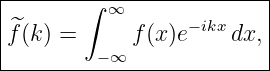
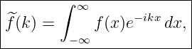
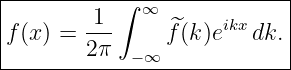
For a continuous one-dimensional field, one useful transform convention is
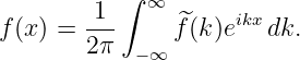
with inverse
A traveling wave packet then has the form
The function
is the wave-number spectrum.
The dispersion relation
controls how each Fourier component evolves.
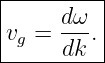
Two velocities then become important:
for the phase velocity, and
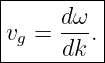
for the group velocity.
When
is nonlinear, different spectral components accumulate phase at different rates and a packet can
broaden or distort. That is dispersion.
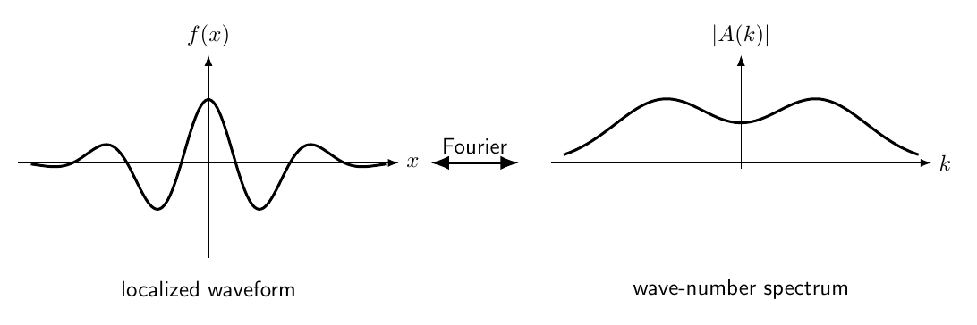
Figure 1. A localized waveform can be regarded as a superposition of many sinusoidal components.
Fourier analysis converts between the spatial waveform and its wave-number spectrum.
1 Why Fourier analysis appears in linear wave physics
The wave equations considered in M06-06 through M06-09 are linear. If
and
are solutions, then
is also a solution for constants
This superposition principle makes sinusoidal modes especially useful.
In translationally invariant systems, complex exponentials
are spatial eigenfunctions. The dynamics of a complicated waveform can therefore be reduced to
the independent evolution of its Fourier components.
2 Fourier series on a finite interval
Suppose
is periodic with period
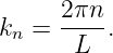
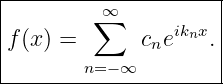
Define
The real Fourier series is
| f(x) | =  + ∑
n=1∞ + ∑
n=1∞![[an cos(knx) + bnsin(knx)]](https://images.physicslibrary.org/cache/objects/1506/make4ht/FourierAnalysisWavePacketsAndDispersion17x.png) . . | (17) |
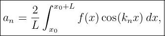
The coefficients are
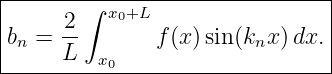
and
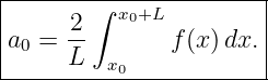
The constant coefficient is
These formulas are direct consequences of sine and cosine orthogonality.
3 Complex Fourier series
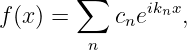
The same periodic function can be written more compactly as
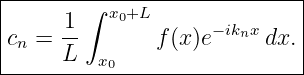
The coefficients are
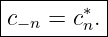
For a real function,
Thus negative wave numbers do not provide independent information for a real field, but they
remain extremely useful in the complex representation.
4 From a Fourier series to a Fourier transform
As the interval becomes very large, the spacing between allowed wave numbers becomes
small:
The discrete sum over
approaches an integral.
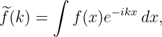
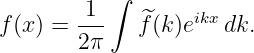
This leads to the Fourier-transform pair
and
A finite-domain normal-mode expansion and an infinite-domain Fourier transform are therefore
closely related versions of the same spectral idea.
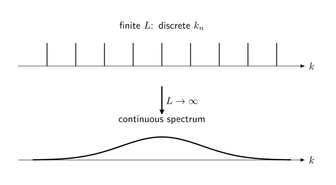
Figure 2. Increasing the spatial period decreases the wave-number spacing Δk = 2π∕L. In the
infinite-domain limit, the discrete Fourier series becomes a continuous Fourier transform.
5 Wave-number spectrum
The function
contains the amplitude and phase of each wave-number component.
A broad waveform in position space often has a narrow spectrum in
while a sharply localized waveform requires a broad range of wave numbers.
This is a general Fourier-localization principle.
6 Gaussian example
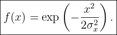
Consider
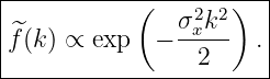
Its Fourier transform is proportional to
Therefore the characteristic spectral width is
for this amplitude-width convention.
A narrow Gaussian in space has a broad Gaussian spectrum, and vice versa.
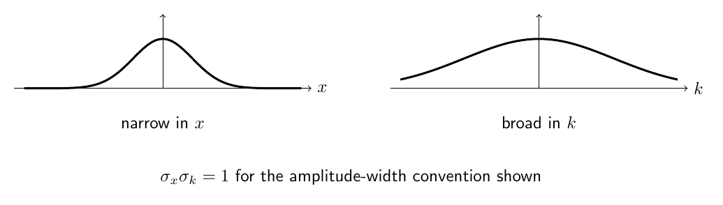
Figure 3. Fourier localization for Gaussian amplitudes. Narrow localization in position requires a
broad wave-number spectrum, while a broad spatial envelope has a narrow spectrum.
7 Standard-deviation localization inequality
If a square-integrable waveform is normalized and standard deviations are defined from
and
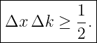
then Fourier analysis gives
A Gaussian attains equality.
This is a purely mathematical Fourier property. It appears in classical wave theory as well as in
quantum mechanics.
8 Parseval relation
The Fourier transform also preserves a quadratic norm. With the transform convention used
here,
This is Parseval’s relation.
It connects total quadratic content in position space with total quadratic content in spectral space.
In wave mechanics, closely related relations underlie modal energy decompositions.
9 A wave packet
A localized wave packet centered near wave number
can be written as
If
is sharply peaked near
then the field resembles a rapidly oscillating carrier multiplied by a slowly varying envelope.
The carrier and envelope need not move at the same velocity.
10 Two nearby waves
Take two waves with nearby wave numbers and frequencies:
and
Their sum is
| y1 + y2 | = 2A cos ![[ ]
(k1-−-k2)x-−-(ω1-−-ω2)t
2](https://images.physicslibrary.org/cache/objects/1506/make4ht/FourierAnalysisWavePacketsAndDispersion43x.png) | |
|
| × cos ![[ ]
(k1 +-k2)x −-(ω1 +-ω2)t
2](https://images.physicslibrary.org/cache/objects/1506/make4ht/FourierAnalysisWavePacketsAndDispersion44x.png) . . | (43) |
Define
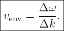
The slowly varying envelope has constant phase when
Therefore its velocity is
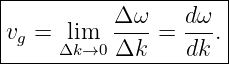
In the narrowband limit,
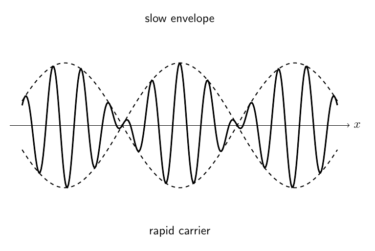
Figure 4. Two nearby Fourier components form a rapidly oscillating carrier inside a slower
envelope. In the narrowband limit the envelope moves at the group velocity dω∕dk.
11 Phase velocity
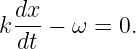
For one Fourier component,
Differentiating,
Therefore
This is the velocity of a constant-phase point such as a crest of an ideal sinusoidal component.
12 Group velocity
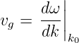
The narrowband envelope moves at
Graphically:
- vp is related to the slope of the line from the origin to the point (k,ω),
- vg is the slope of the tangent to the dispersion curve at that point.
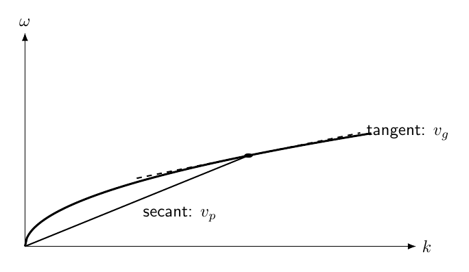
Figure 5. On a dispersion diagram, phase velocity is the secant slope ω∕k from the origin, while
group velocity is the local tangent slope dω∕dk.
13 Carrier-envelope form
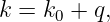
Let
where
is small for a narrow spectrum.
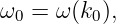
Expand the frequency:
| ω(k) | = ω0 + ω0′q +  ω0′′q2 + ω0′′q2 +  , , | (54) |
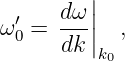
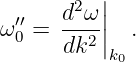
where
and
If the quadratic and higher terms are neglected, the packet becomes
where
Thus the carrier oscillates at
while the envelope translates at the group velocity.
14 Nondispersive medium
If
for positive
then
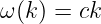
Also,
All Fourier components advance with compatible phase evolution. An ideal packet can translate
without dispersive broadening.
The ideal stretched string in M06-08 is nondispersive within its linear model.
15 Dispersive medium
A medium is dispersive when
is nonlinear.
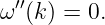
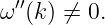
Then, in general,
and
Different Fourier components acquire different relative phases as time evolves. This can change the
packet shape.
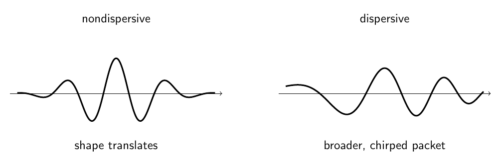
Figure 6. In a nondispersive medium a localized envelope translates without changing its spectral
phase relationships. In a dispersive medium different wave-number components accumulate
different phases and the packet broadens or distorts.
16 Second-order dispersion and packet broadening
For a narrow spectrum, retain the quadratic term:
| ω(k) | ≈ ω0 + vgq +  ω0′′q2. ω0′′q2. | (68) |
The linear term translates the envelope.
The quadratic term produces spreading.
For a Gaussian spectral amplitude
the amplitude envelope remains Gaussian under this quadratic approximation.
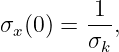
If its initial amplitude width is
then
The sign of
affects the spectral phase chirp, while the width depends on its magnitude in this simple Gaussian
result.
17 Example 1: Gaussian spreading
Suppose
Then
Let
After
| σx(t) | = 0.500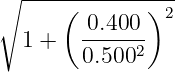 | (77)
|
| ≈ 0.943 mm. | (78) |
The packet has nearly doubled its characteristic amplitude width.
18 Example 2: monatomic oscillator chain
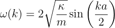
M06-06 found
for
Take
At
The angular frequency is
| ω | = 40 sin  | (84)
|
| ≈ 28.28 mrad∕s. | (85) |
The phase velocity is
| vp | =  | (86)
|
| ≈ 1.80 mm∕s. | (87) |
The group velocity is
| vg | = a cos cos  | (88)
|
| = 2.00 cos  | (89)
|
| ≈ 1.41 mm∕s. | (90) |
Thus
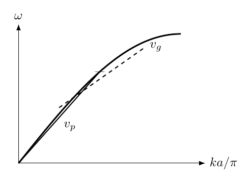
Figure 7. On the monatomic-chain dispersion curve, the secant and tangent slopes differ away
from the long-wavelength limit. The packet envelope therefore travels at a different speed from
the carrier phase.
19 Spectral evolution is especially simple
Suppose the initial spectrum is
For a linear time-invariant wave system with dispersion relation
each component simply acquires a phase factor:
The spectral magnitude is unchanged:
Dispersion changes the relative spectral phases. Those phase changes alter the waveform after
transforming back to position space.
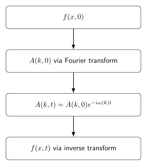
Figure 8. Linear propagation leaves the magnitude of each spectral component unchanged but
advances its phase by −ω(k)t. A nonlinear dispersion relation causes the accumulated phase to
vary nonlinearly across the spectrum.
20 Initial-value propagation by Fourier transform
A common wave-analysis workflow is:
- Fourier transform the initial field to obtain its spectral amplitudes.
- Multiply each spectral component by its propagation phase factor.
- Inverse transform to reconstruct the field at the desired time.
Schematically,
This is the continuous-wave analogue of propagating independent normal coordinates in a
finite-dimensional system.
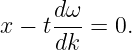
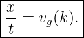
21 Stationary-phase interpretation of group velocity
At large distance and time, rapidly varying phases tend to cancel under integration. The
strongest contribution often comes from wave numbers where the total phase varies
slowly.
For phase
stationary phase requires
Therefore
Hence the dominant wave number contributing along the ray
satisfies
This gives a deeper asymptotic interpretation of group velocity.
22 Group velocity and energy transport
In many conservative weakly dispersive systems, wave-packet energy is transported approximately
at the group velocity.
This statement is powerful but should not be used mechanically in every possible medium.
Absorption, strong inhomogeneity, active media, and unusual dispersion can require a more careful
energy-flux analysis.
For the ideal conservative systems developed in this mechanics sequence, group velocity is the
natural velocity associated with a narrowband packet envelope and usually with its transported
energy.
23 Negative group velocity and sign conventions
The derivative
can be negative on some branches or for some sign conventions.
That does not mean the mathematical framework has failed. It means the local slope of the
dispersion curve is negative.
The physical interpretation must be made using the full wave field, energy flux, and the chosen
representation of positive and negative wave numbers.
24 Finite bandwidth matters
The approximation
works best when the spectrum is sufficiently narrow that the dispersion curve is nearly linear
across the occupied bandwidth.
If the spectrum is broad, one group velocity cannot describe the entire packet. Higher derivatives
such as
become important.
25 Connection to normal modes
On a finite string, the wave numbers are discrete and the field is expanded in normal
modes:
On an infinite or very long translationally invariant medium, the spectrum becomes
continuous:
The mathematical transition is
The physical idea is the same: decompose the motion into independent linear modes.
26 Common mistakes
- Confusing Fourier-series coefficients with Fourier-transform amplitudes.
- Mixing transform conventions without carrying the correct factors of 2π.
- Treating a localized pulse as a single wave number.
- Assuming a narrow spatial pulse has a narrow wave-number spectrum.
- Confusing the phase velocity ω∕k with the group velocity dω∕dk.
- Assuming vp = vg in every medium.
- Calling every medium dispersive merely because it supports waves.
- Forgetting that dispersion is controlled by the nonlinearity of ω(k).
- Assuming a wave packet cannot change shape if its spectral magnitudes are constant.
- Forgetting that relative spectral phase is enough to reshape the packet.
- Using one group velocity for a packet whose bandwidth is too broad for linearization
of ω(k).
- Forgetting that ω′′ controls leading-order packet spreading near k0.
- Interpreting the Fourier localization inequality as exclusively quantum mechanical.
- Forgetting conjugate symmetry c−n = cn∗ for a real field.
- Assuming a negative group velocity can be interpreted safely without checking the full
energy-flow problem.
27 Practice exercises
- Derive the real Fourier coefficients from sine and cosine orthogonality.
- Derive the complex Fourier coefficient formula.
- Show how Δk = 2π∕L approaches a continuous spectrum as L →∞.
- Compute the Fourier transform of a Gaussian and identify its spectral width.
- Verify Parseval’s relation for a Gaussian using the transform convention in this article.
- Derive the two-wave envelope formula and the finite-difference envelope velocity
Δω∕Δk.
- Take the narrowband limit and obtain vg = dω∕dk.
- Derive the carrier-envelope form by expanding ω(k) about k0 to first order.
- Show that a linear dispersion relation gives vp = vg and no second-order dispersive
spreading.
- Derive the Gaussian packet-width formula using a quadratic expansion of ω(k).
- Reproduce the Gaussian spreading example.
- Reproduce the monatomic-chain phase and group velocities in Example 2.
- Show that linear propagation preserves |A(k)| while changing spectral phase.
- Derive the stationary-phase condition x∕t = dω∕dk.
- Explain how Fourier decomposition on an infinite domain generalizes the normal-mode
decomposition of a finite string.
28 Summary
A periodic waveform can be expanded as a Fourier series,
while an infinite-domain waveform can be represented by the Fourier transform pair
and
A wave packet is a superposition
The phase velocity is
and the group velocity is
A linear dispersion relation is nondispersive. A nonlinear dispersion relation generally causes
different spectral components to accumulate different relative phases.
For a narrowband Gaussian packet, the second derivative
controls the leading-order broadening.
Fourier analysis therefore unifies normal modes, traveling waves, localized packets, and dispersion
within one spectral framework.
References
References
[1] PhysicsLibrary, M06-09, Waves on Strings: Reflection, Transmission, and Mechanical
Impedance.
[2] PhysicsLibrary, M06-08, Continuous Strings, Standing Waves, and Normal Modes.
[3] PhysicsLibrary, M06-06, Discrete Oscillator Chains and Dispersion.
[4] A. P. French, Vibrations and Waves, W. W. Norton, 1971.
[5] J. R. Taylor, Classical Mechanics, University Science Books, 2005.
[6] R. N. Bracewell, The Fourier Transform and Its Applications, 3rd ed., McGraw-Hill,
2000.

![|-----------------------------------|
| 1 ∫ ∞ |
ψ (x,t) = --- A(k)ei[kx−ω(k)t]dk. |
----------2π--−∞---------------------](https://images.physicslibrary.org/cache/objects/1506/make4ht/FourierAnalysisWavePacketsAndDispersion2x.png)










![|------------∫--------------------|
| 1-- i[kx−ω(k)t] |
ψ (x,t) = 2π A(k)e dk. |
-----------------------------------](https://images.physicslibrary.org/cache/objects/1506/make4ht/FourierAnalysisWavePacketsAndDispersion38x.png)
















![[ ]
(k-−-k0)2
A(k) ∝ exp − 2σ2 ,
k](https://images.physicslibrary.org/cache/objects/1506/make4ht/FourierAnalysisWavePacketsAndDispersion71x.png)
![|------------∘----------------|
| [ ′′ ]2 |
σx (t) = σx(0) 1 + -ω0t-- . |
| σ2x(0) |
------------------------------](https://images.physicslibrary.org/cache/objects/1506/make4ht/FourierAnalysisWavePacketsAndDispersion73x.png)






















![|---------------------------------|
| 1 ∫ |
ψ (x,t) = --- A(k)ei[kx−ω(k)t]dk. |
----------2π-----------------------](https://images.physicslibrary.org/cache/objects/1506/make4ht/FourierAnalysisWavePacketsAndDispersion110x.png)