Physics Library
 An open source physics library
Encyclopedia | Forums | Docs | Random  
[parent] Calculus of Variations: Computing Second Variations - Exercises

(Example)

Calculus of Variations: Computing Second Variations - Exercises and Worked Solutions

CV11 introduced the second variation as the variational analogue of a Hessian quadratic form. This companion entry is deliberately computational. The goal is to become fluent at moving between three equivalent viewpoints:

Φ η(𝜖) = J[y∗ + 𝜖η ],
(1)

              2      |
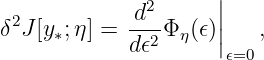
δ2J[y ;η] = -d-Φ  (𝜖)||   ,
     ∗      d𝜖2  η   |𝜖=0
(2)

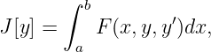
and, for a first-order functional J[y] = ∫ abF(x,y,y′)dx,

|------------------------------------------------|
|           ∫  b(                           )    |
|δ2J[y∗;η] =     Fyyη2 + 2Fyy′ηη′ + Fy′y′(η′)2  dx .
--------------a----------------------------------
(3)

All derivatives of F are evaluated along the candidate y∗. The main lesson emphasized that this quadratic form carries classification information only after y∗ has first been shown to be stationary. The exercises below reinforce that separation. Standard treatments of the second variation and Legendre condition include [1, 2, 3, 4].

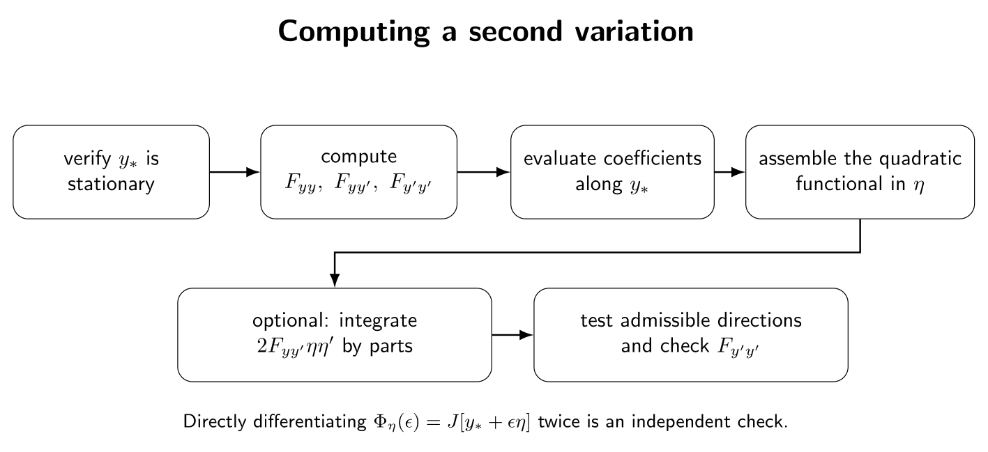
PIC

Figure. A reliable workflow for computing the second variation. Direct epsilon differentiation and Hessian-coefficient assembly must give the same quadratic functional.

1 Exercises

Exercise 1: a positive quadratic functional

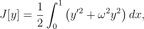
Consider

         ∫  1
J [y] = 1-   (y′2 + ω2y2 )dx,     y(0) = y(1) = 0,
        2  0
(4)

where ω is a real constant.

  1. Verify that y∗(x) = 0 is stationary.
  2. Compute δ2J[0; η] from the Hessian formula.
  3. Evaluate the result for η(x) = sin(πx).

Exercise 2: direct epsilon expansion with variable coefficients

Let

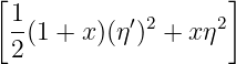
          [                  ]
       ∫ 1  1        ′2     2
J[y] =      -(1 + x)y  + xy   dx.
        0   2
(5)

For a general candidate y∗ and variation η:

  1. substitute y∗ + 𝜖η directly and isolate the coefficient of 𝜖2;
  2. infer δ2J[y ∗; η];
  3. check the result using Fyy, Fyy′, and Fy′y′;
  4. evaluate it for η = x(1 − x).

Exercise 3: a mixed term that becomes a boundary term

Consider

      ∫  1[1             β   ]
J[y] =     --y′2 + αyy ′ +--y2  dx,
        0  2             2
(6)

with fixed endpoints y(0) = y(1) = 0.

  1. Compute the three Hessian coefficients.
  2. Write the unreduced second variation.
  3. Show explicitly that the mixed term integrates to zero for admissible variations.
  4. Evaluate the reduced form for η = sin(πx).

Exercise 4: a nontrivial stationary logarithmic extremal

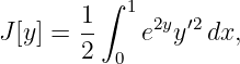
Consider

       1 ∫ 1
J[y] = --   e2yy′2dx,
       2  0
(7)

with endpoint values

y(0) = 0,     y(1) = ln2.
(8)

  1. Verify that
    y∗(x) = ln(1 + x)
    (9)

    is an Euler–Lagrange extremal.

  2. Compute Fyy, Fyy′, and Fy′y′ along y∗.
  3. Write the unreduced second variation.
  4. Integrate the mixed term by parts and show that the η2 term cancels completely.

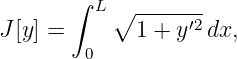
Exercise 5: second variation of arc length about a straight line

For

       ∫
         L ∘ -----′2
J [y] =       1 + y  dx,
        0
(10)

let

y∗(x) = mx  + b
(11)

join the prescribed endpoints.

  1. Compute the second variation about y∗.
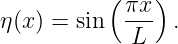
  2. Evaluate it for
              ( πx-)
η(x) = sin   L   .
    (12)

  3. State what the sign tells you and what it does not prove by itself.

Exercise 6: harmonic-oscillator action and trial modes

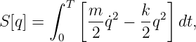
For the mechanical action

       ∫ T [           ]
S [q] =      m-q˙2 − k-q2  dt,
        0    2      2
(13)

let q∗ be any stationary trajectory with fixed endpoints.

  1. Compute δ2S[q ∗; η].
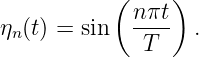
  2. Evaluate it on the trial family
               ( nπt )
ηn(t) = sin   ----  .
              T
    (14)

  3. For each n, find the interval length at which this particular trial direction becomes neutral.

Exercise 7: a nonlinear slope energy and the Legendre coefficient

Let

       ∫  [                   ]
         b  1 ′4   α  ′2
J [y] =      -y  +  -y  +  V (y ) dx.
        a   4      2
(15)

  1. Compute the second variation about a stationary function y∗.
  2. Identify the Legendre coefficient Fy′y′.
  3. If y∗ = 0 is stationary and V ′(0) = 0, simplify the result.
  4. Explain immediately why α < 0 rules out y∗ = 0 as a weak local minimum.

Exercise 8: a variable-coefficient quadratic form

Consider

        ∫  1
J[y] = 1-   [(1 + x)y′2 − λy2 ]dx,     y(0) = y(1) = 0.
       2  0
(16)

  1. Show that y∗ = 0 is stationary and compute its second variation.
  2. Evaluate the second variation on η = sin(πx).
  3. Find the values of λ for which this one trial direction already proves that y∗ = 0 cannot be a local minimum.

Exercise 9: the bilinear variational Hessian

For

         ∫ 1
J[y] = 1-   (y′2 + ω2y2)dx,
       2  0
(17)

define

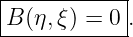
B (η,ξ) = δ2J [0;η, ξ].
(18)

  1. Compute B(η,ξ).
  2. Verify explicitly that B(η,ξ) = B(ξ,η).
  3. Evaluate B for
    η = sin (πx),     ξ = sin(2πx ).
    (19)

  4. Explain the relation between B(η,η) and the ordinary second variation.

2 Worked solutions

Solution 1: a positive quadratic functional

The integrand is

      ′    1(  ′2    2 2)
F (y,y ) = 2 y  +  ω y   .
(20)

Its first derivatives are

Fy =  ω2y,     Fy′ = y′.
(21)

At y∗ = 0, both vanish, so the Euler–Lagrange equation is satisfied. The Hessian coefficients are

        2
Fyy =  ω ,    Fyy ′ = 0,    Fy′y′ = 1.
(22)

Therefore

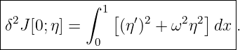
|-----------∫-1-----------------|
|δ2J[0;η] =    [(η′)2 + ω2 η2]dx .
-------------0-------------------
(23)

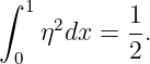
For η = sin(πx),

η ′ = π cos(πx),
(24)

and

∫                ∫
   1   2            1   2          1-
    sin  (πx )dx =     cos (πx)dx =  2.
  0                0
(25)

Hence

|-------------------(-------)-|
|δ2J [0;sin(πx )] = 1- π2 + ω2  .
------------------2-----------|
(26)

This is strictly positive for every real ω and every nonzero version of this trial direction.

Solution 2: direct epsilon expansion with variable coefficients

Substitute

y𝜖 = y ∗ + 𝜖η,   y′𝜖 = y′∗ + 𝜖η′.
(27)

Then

J[y𝜖] = ∫ 01[                                ]
 1-(1 + x )(y ′+ 𝜖η′)2 + x (y + 𝜖η)2
 2         ∗              ∗dx (28)
= J[y∗] + 𝜖∫ 01[(1 + x)y′∗η′ + 2xy∗η] dx (29)
+ 𝜖2 ∫ 01[                   ]
 1-         ′2     2
 2 (1 + x)(η)  + xηdx. (30)

Because the Taylor convention is

                           𝜖2 2
J [y∗ + 𝜖η] = J[y∗] + 𝜖δJ + 2 δ J + ⋅⋅⋅ ,
(31)

we obtain

|------------∫-1------------------------|
|δ2J[y ;η] =    [(1 + x)(η′)2 + 2x η2]dx .
|     ∗       0                         |
----------------------------------------
(32)

The Hessian check gives

Fyy =  2x,    Fyy ′ = 0,    Fy′y′ = 1 + x,
(33)

which reproduces the same result.

For

                   ′
η = x(1 − x),     η = 1 − 2x,
(34)

we find

δ2J = ∫ 01[                             ]
 (1 + x )(1 − 2x )2 + 2x3(1 − x)2dx (35)
= -8-
15 . (36)

This example is useful because the second variation does not depend on y∗ at all: the original functional is already quadratic in y and y′.

Solution 3: a mixed term that becomes a boundary term

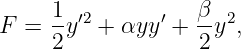
For

     1- ′2      ′   β- 2
F =  2y  +  αyy +  2 y ,
(37)

we have

Fyy = β,     Fyy′ = α,     Fy′y′ = 1.
(38)

Therefore

      ∫ 1
 2        [  2        ′    ′2]
δ J =  0  β η +  2αηη  + (η )  dx.
(39)

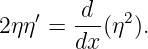
Now use

2 ηη′ = d-(η2).
        dx
(40)

Thus

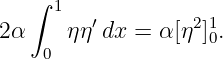
   ∫ 1
2α    η η′dx = α [η2]10.
    0
(41)

Because admissible fixed-endpoint variations satisfy

η(0) = η(1) = 0,
(42)

this boundary contribution vanishes. Hence

|------∫-1-----------------|
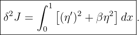
|δ2J =     [(η ′)2 + βη2] dx .
|       0                  |
---------------------------
(43)

For η = sin(πx),

|----------------|
|2     1- 2      |
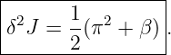
δ J =  2(π  + β ).
------------------
(44)

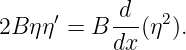
Notice that α disappears completely from the fixed-endpoint second variation. In fact, αyy′ = α-
2(d∕dx)(y2) is itself a total derivative.

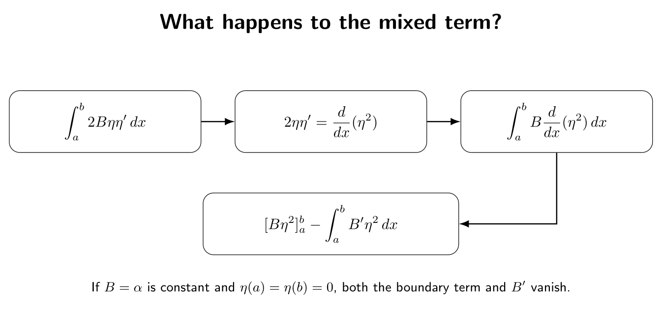
PIC

Figure. The mixed term 2Fyy′ηη′ can often be converted into an η2 contribution plus an endpoint term. For constant Fyy′ = α and fixed endpoints, only the boundary term remains, and it vanishes.

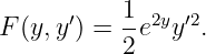
Solution 4: a nontrivial stationary logarithmic extremal

Here

F(y,y ′) = 1-e2yy ′2.
          2
(45)

The first derivatives are

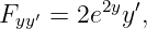
      2y ′2       ′    2y ′
Fy = e  y  ,    Fy  = e  y .
(46)

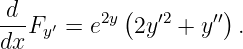
Therefore

 d        2y (  ′2   ′′)

---Fy′ = e   2y  + y   .
dx
(47)

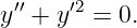
The Euler–Lagrange equation becomes

 ′′    ′2
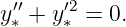
y + y   = 0.
(48)

For

y ∗ = ln(1 + x),
(49)

we have

y′=  --1--,     y′′ = − ---1----,
 ∗   1 + x       ∗     (1 + x)2
(50)

so indeed

 ′′    ′2
y∗ + y ∗ = 0.
(51)

The second derivatives of F are

Fyy = 2e2yy′2,
(52)

Fyy′ = 2e2yy′,
(53)

and

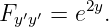
Fy ′y′ = e2y.
(54)

Along y∗ = ln(1 + x),

e2y∗ = (1 + x )2,
(55)

and therefore

F   = 2,     F  ′ = 2(1 + x),    F  ′′ = (1 + x )2.
  yy            yy                   yy
(56)

The unreduced form is

      ∫  1[                                ]
δ2J =      2η2 + 4(1 + x)ηη′ + (1 + x )2(η′)2 dx.
        0
(57)

Since

4(1 + x)ηη′ = 2(1 + x)-d-(η2),
                      dx
(58)

integration by parts gives

∫  1                                  ∫ 1
    4(1 + x)ηη′dx =  [2(1 + x)η2]1−  2    η2dx.
  0                              0     0
(59)

The boundary term vanishes, so the −2η2 produced here cancels the original +2η2. Thus

|-----------∫--1---------------|
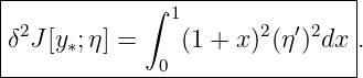
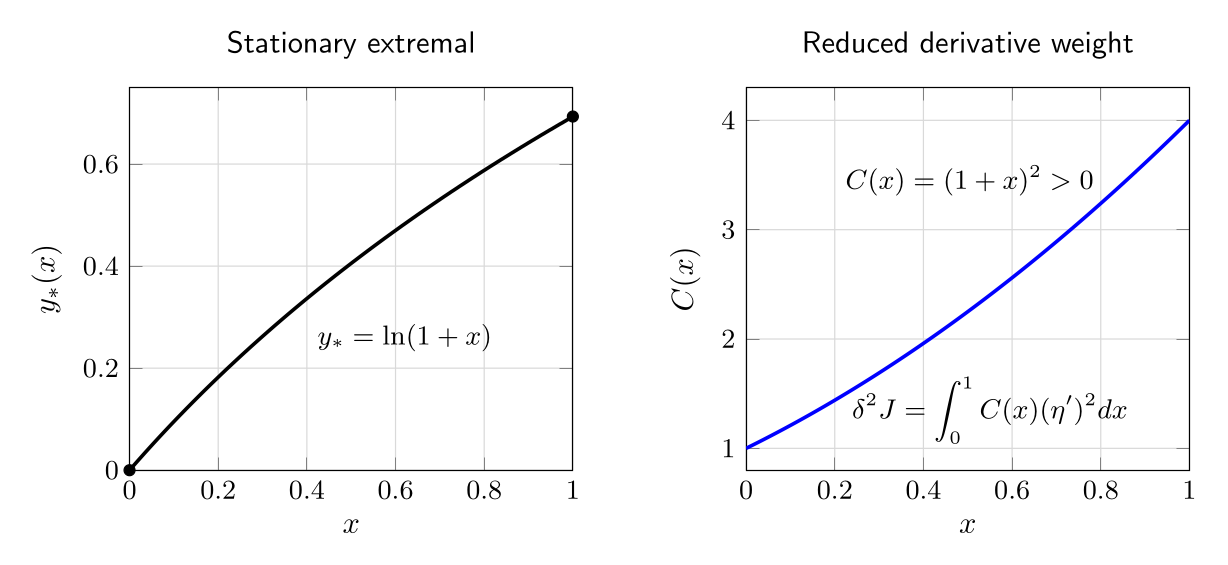
δ2J [y ;η] =    (1 + x )2(η′)2dx .
|     ∗       0                |
-------------------------------
(60)

This is a useful example because a complicated-looking Hessian quadratic form collapses to a manifestly nonnegative expression after the mixed term is handled correctly.

PIC

Figure. The stationary curve y∗ = ln(1 + x) and the positive Weight (1 + x)2 appearing in its reduced second variation.

Solution 5: second variation of arc length about a straight line

For

    ′   ∘ -----′2
F (y ) =   1 + y  ,
(61)

we have

Fy = 0,     Fyy = 0,     Fyy′ = 0.
(62)

Also,

      ---y-′---
Fy′ = ∘1--+-y′2,
(63)

so

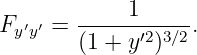
        ----1------
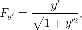
Fy′y′ = (1 + y ′2)3∕2 .
(64)

Along the straight line y∗′ = m,

|-----------------------∫-L--------|
δ2J [y ;η ] =-----1------   (η ′)2dx .
|    ∗      (1 + m2 )3∕2  0         |
------------------------------------
(65)

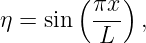
For

       (πx-)
η = sin   L   ,
(66)

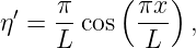
we have

 ′   π-   ( πx-)
η =  L cos   L   ,
(67)

and therefore

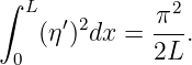
∫ L            2
    (η ′)2dx =  π-.
 0            2L
(68)

Hence

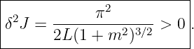
|-------------------------|
| 2          π2           |
|δ J =  ---------2-3∕2->  0.
--------2L(1-+-m--)-------
(69)

This positive value confirms positive curvature of the functional along this trial direction. Positivity in one direction alone does not prove a minimum. Here the full quadratic form is positive for every nonzero fixed-endpoint variation, which is much stronger; a complete sufficiency statement still belongs to the later theory.

Solution 6: harmonic-oscillator action and trial modes

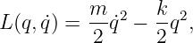
For

L (q, ˙q) = m-˙q2 − kq2,
          2      2
(70)

we have

Lqq =  − k,    Lqq˙= 0,     Lq˙q˙= m.
(71)

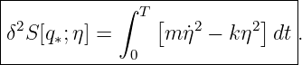
Thus every stationary trajectory has the same second variation,

|-----------∫-T----------------|
δ2S [q ;η] =     [m ˙η2 − kη2]dt .
|    ∗       0                 |
--------------------------------
(72)

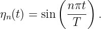
Take

           ( nπt )
ηn(t) = sin   ----  .
              T
(73)

Then

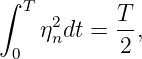
∫ T
     2     T-
 0  ηndt = 2 ,
(74)

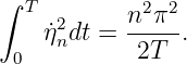
and

∫
   T 2      n2π2-
    η˙ndt =  2T  .
  0
(75)

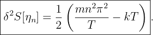
Therefore

|-----------(----2--2------)-|
δ2S [η ] = 1- mn--π--−  kT   .
|     n    2     T           |
------------------------------
(76)

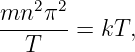
This direction becomes neutral when

mn2-π2-
   T    = kT,
(77)

or

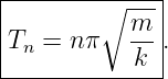
|--------∘----|
|T  = n π   m-.
| n         k |
---------------
(78)

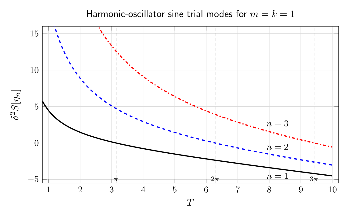
For T > Tn, that trial direction produces a negative second variation. The first mode n = 1 therefore detects loss of positive definiteness first. This is the calculation behind the conjugate-point threshold developed more systematically in CV12 and is standard in variational mechanics [5, 1].

PIC

Figure. Second variation of the first three sine trial modes as the endpoint separation T changes, with m = k = 1. Each mode crosses zero at Tn = nπ.

Solution 7: a nonlinear slope energy and the Legendre coefficient

The integrand is

      ′   1- ′4   α- ′2
F(y, y) = 4 y  + 2 y  + V (y).
(79)

Its relevant second derivatives are

        ′′
Fyy = V  (y),    Fyy′ = 0,
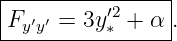
(80)

and

         ′2
Fy′y′ = 3y  + α.
(81)

Therefore about a stationary y∗,

|----------------------------------------------|
|           ∫ b [           (        )     ]   |

δ2J [y∗;η] =      V′′(y∗)η2 +  3y′∗2+ α  (η′)2 dx .
-------------a----------------------------------
(82)

The Legendre coefficient is

|---------------|
|Fy′y′ = 3y′∗2+ α |.
-----------------
(83)

If y∗ = 0 is stationary, then V ′(0) = 0 and y∗′ = 0, so

|-----------∫------------------------|
| 2           b[  ′′    2      ′2]    |
|δ J[0;η] =     V  (0)η + α (η)   dx .
-------------a-----------------------
(84)

If α < 0, then

Fy′y′ = α < 0
(85)

along the candidate. The Legendre necessary condition for a weak local minimum is violated immediately. No further classification calculation is needed to rule out a weak minimum.

Solution 8: a variable-coefficient quadratic form

The functional is already quadratic, and y∗ = 0 plainly satisfies the Euler–Lagrange equation. The Hessian coefficients are

Fyy = − λ,     Fyy′ = 0,    Fy′y′ = 1 + x.
(86)

Hence

|-----------∫-1-----------------------|
|δ2J[0;η] =    [(1 + x)(η′)2 − λ η2]dx .
|            0                        |
---------------------------------------
(87)

For η = sin(πx),

∫
  1  2     1-
    η dx = 2 .
 0
(88)

Also,

  ′
η  = π cos(πx),
(89)

so

∫ 01(1 + x)(η′)2dx = π2 ∫ 01(1 + x) cos 2(πx)dx (90)
= 3π2-
 4. (91)

Therefore

|--------------------------|
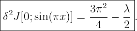
| 2               3π2-  λ- |
|δ J[0;sin (πx )] =  4  −  2 .
---------------------------
(92)

This trial direction is negative when

     3π2-
λ >   2 .
(93)

Thus

|------2---------------------------------------|
λ >  3π--  = ⇒    0 cannot be a local minimum   .
------2-----------------------------------------
(94)

This is only a one-direction test. If the value is positive, we have not proved that the quadratic form is positive for every admissible variation.

Solution 9: the bilinear variational Hessian

For the quadratic functional,

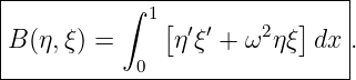
|-----------------------------|
|          ∫ 1[           ]   |
|B (η,ξ) =     η′ξ′ + ω2 ηξ dx .
------------0------------------
(95)

The integrand is unchanged when η and ξ are interchanged, so

|-----------------|
|B (η,ξ) = B (ξ, η).
------------------
(96)

Now choose

η = sin (πx),     ξ = sin(2πx ).
(97)

Orthogonality gives

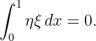
∫ 1
   η ξdx =  0.
 0
(98)

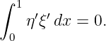
Their derivatives are proportional to cos(πx) and cos(2πx), which are also orthogonal on [0, 1], so

∫
   1 ′ ′
    η ξ dx = 0.
  0
(99)

Hence

|-----------|
-B-(η,ξ) =-0 .
(100)

Finally, the ordinary quadratic second variation is simply the bilinear Hessian evaluated twice in the same direction:

|------------------|
δ2J [0; η] = B (η,η) .
--------------------
(101)

This is exactly analogous to the finite-dimensional expression hT Hh obtained by inserting the same displacement vector into both slots of the Hessian bilinear form.

3 A compact computation checklist

For a functional

       ∫ b
J [y] =    F (x,y,y ′)dx,
        a
(102)

a reliable calculation proceeds as follows.

  1. Verify that the candidate is stationary before using the second variation for classification.
  2. Compute
    A  = F  ,     B =  F  ′,     C =  F ′′
      yy            yy            yy
    (103)

    along the candidate.

  3. Assemble
           ∫
 2           2        ′     ′2
δ J =    (Aη  + 2B ηη  + C η )dx.
    (104)

  4. If useful, reduce the mixed term using
         ′     d-- 2
2B ηη = B  dx(η ).
    (105)

  5. Apply the actual endpoint conditions before discarding boundary terms.
  6. Check the Legendre coefficient C = Fy′y′.
  7. Evaluate selected trial functions to find negative or neutral directions.
  8. Do not infer positivity for all variations from positivity on only one or a few trial directions.

The last point is the bridge to CV11E2 and CV12: computing a quadratic form is straightforward; proving its sign for an infinite-dimensional class is the deeper problem.

4 Summary

The second variation can be obtained either by direct epsilon expansion or by differentiating the integrand Hessian. For fixed-endpoint problems the general expression is

       ∫
 2       b(     2         ′        ′2)

δ J =      Fyyη  + 2Fyy′ηη  + Fy′y′η   dx.
        a
(106)

The mixed term often simplifies after integration by parts, but it must not simply be dropped. The Legendre coefficient Fy′y′ gives a pointwise necessary condition, while selected trial directions can disprove minimality by producing a negative second variation. Positive values on a few directions are not a proof of a minimum. That distinction motivates the classification and Jacobi-field problems that follow.

References

[1]   I. M. Gelfand and S. V. Fomin, Calculus of Variations, Dover Publications, 2000.

[2]   Bruce van Brunt, The Calculus of Variations, Springer, 2004.

[3]   Hans Sagan, Introduction to the Calculus of Variations, Dover Publications, 1992.

[4]   Robert Weinstock, Calculus of Variations with Applications to Physics and Engineering, Dover Publications, 1974.

[5]   Cornelius Lanczos, The Variational Principles of Mechanics, Dover Publications, 1986.


"Calculus of Variations: Computing Second Variations - Exercises" is owned by bloftin.
(view preamble)
View style:
Other names:  CV11E1
Keywords:  calculus of variations, second variation, variational Hessian, quadratic form, Legendre condition, mixed term, accessory functional, arc length, harmonic oscillator, stationary function, trial variation

This object's parent.

Cross-references: vector, displacement, mechanics, CV12, detects, Weight, boundary, relation, function, formula, Legendre condition, second variation, CV11

This is version 1 of Calculus of Variations: Computing Second Variations - Exercises, born on 2026-10-20.
Object id is 1513, canonical name is CalculusOfVariationsComputingSecondVariationsExercises.
Accessed 11 times total.

Classification:
Physics Classification: 02.30.Xx (Calculus of variations)
 02.30.Sa (Functional analysis)
 45.20.Jj (Lagrangian and Hamiltonian mechanics)
 42.15.-i (Geometrical optics)

Pending Errata and Addenda

None.

Discussion

No messages.

Interact