Electromagnetic Waves, Antennas, and RF: Electric Charge and the Electric Field - Exercises and
Complete Worked Solutions
This companion article provides self-study exercises for EM05, Electric Charge and the
electric field. All exercises are stated first. Complete worked solutions follow in Part
II.
The problems reinforce the central ideas introduced in EM05: charge sign and quantization,
Coulomb’s law, source-to-observation geometry, the test-charge definition of electric field, the field
of a point charge, inverse-square scaling, and vector superposition.
The elementary charge magnitude is
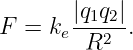
Coulomb’s law for two stationary point charges is
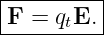
The electric field is defined by
or equivalently
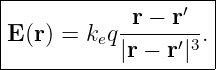
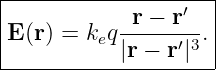
For a point charge q at source point r′, the field at observation point r is
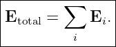
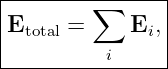
Electric fields superpose linearly:
These are the same definitions and conventions used in EM05 [1, 2, 3, 5].
How to use this problem set
Attempt all exercises in Part I before reading Part II. In vector problems, keep the following
sequence explicit:
- identify source and observation locations;
- form R = r − r′;
- determine the magnitude R and unit vector R;
- apply the sign of the source charge correctly;
- add field vectors component by component.
Part I: Exercises
Exercise 1: charge quantization
An isolated object has net charge
How many excess electrons does this charge represent? State the sign interpretation
clearly.
Exercise 2: Coulomb-force magnitude and sign
Two point charges are separated by
Their charges are
Find the magnitude of the electrostatic force and state whether the interaction is attractive or
repulsive.
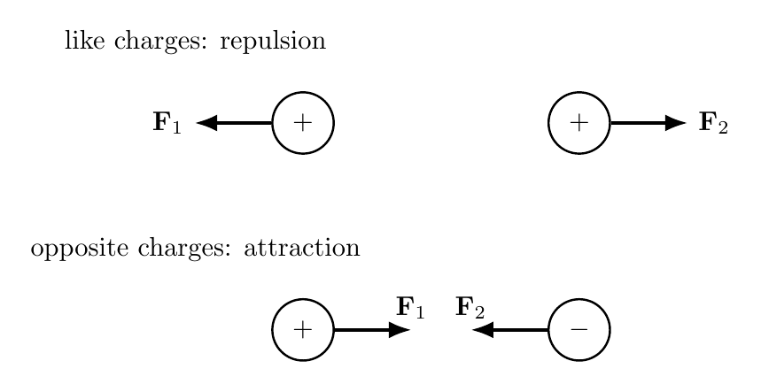
Figure. Like signs repel and unlike signs attract. The force directions follow from charge
sign, while Coulomb’s law gives the magnitude.
Exercise 3: vector Coulomb force from coordinates
A source charge
is located at
and a second charge
is located at
Find the force on q2 due to q1 in Cartesian-vector form.
Exercise 4: source point, observation point, and separation vector
A point charge is located at
The observation point is
Find:
- R = r − r′;
- R = |R|;
- R.
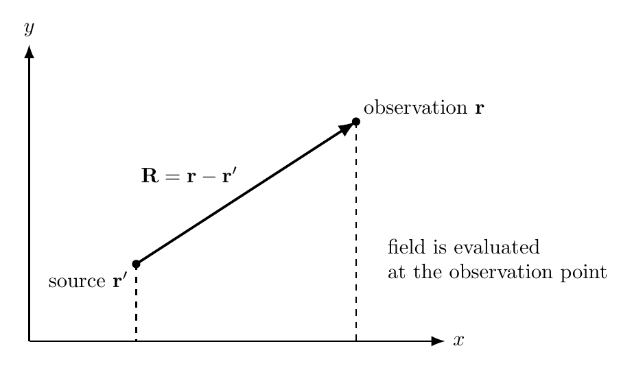
Figure. The source point r′ and observation point r are connected by R = r − r′.
Exercise 5: field magnitude and direction from a negative point charge
A point charge
is at the origin. Find the electric-field magnitude at a distance
and state the field direction relative to the source charge.
Exercise 6: force on a negative test charge
At a point in space,
A test charge
is placed at that point.
Find the force vector and its magnitude. Explain why the force direction is opposite the
electric-field direction.
Exercise 7: cancellation by symmetry
Two identical positive charges +q are placed at
Find the total electric field at the origin. Explain the cancellation using both magnitude and
direction.
Exercise 8: two-dimensional vector superposition
At an observation point P, two sources produce
and a second field of magnitude
at an angle of 120∘ counterclockwise from the +x axis.
Find the total field in Cartesian form, its magnitude, and its direction measured counterclockwise
from +x.
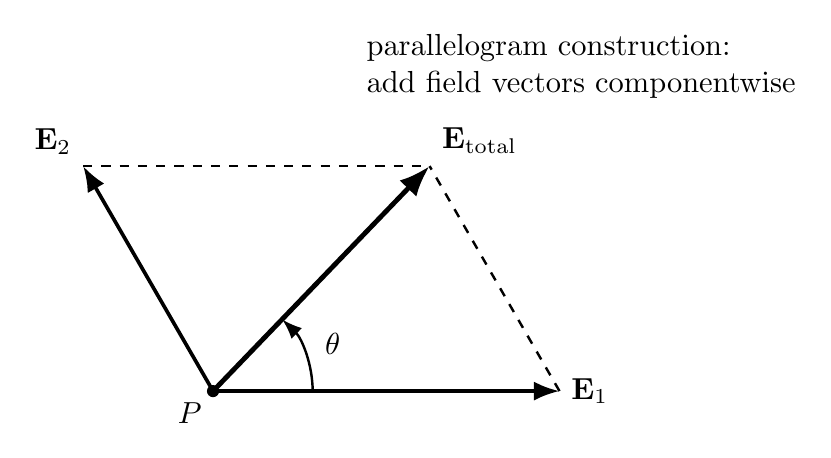
Figure. Electric-field superposition is vector addition at the common observation point.
Exercise 9: opposite charges and a midpoint field
A charge
is located at x = −0.20 m, and a charge
is located at x = +0.20 m.
Find the total electric field at the origin. State its direction.
Exercise 10: inverse-square scaling
A point charge produces field magnitude E1 at distance r1.
Find E2∕E1 when
Then find the distance ratio r2∕r1 required to reduce the field magnitude to one ninth of its
original value.
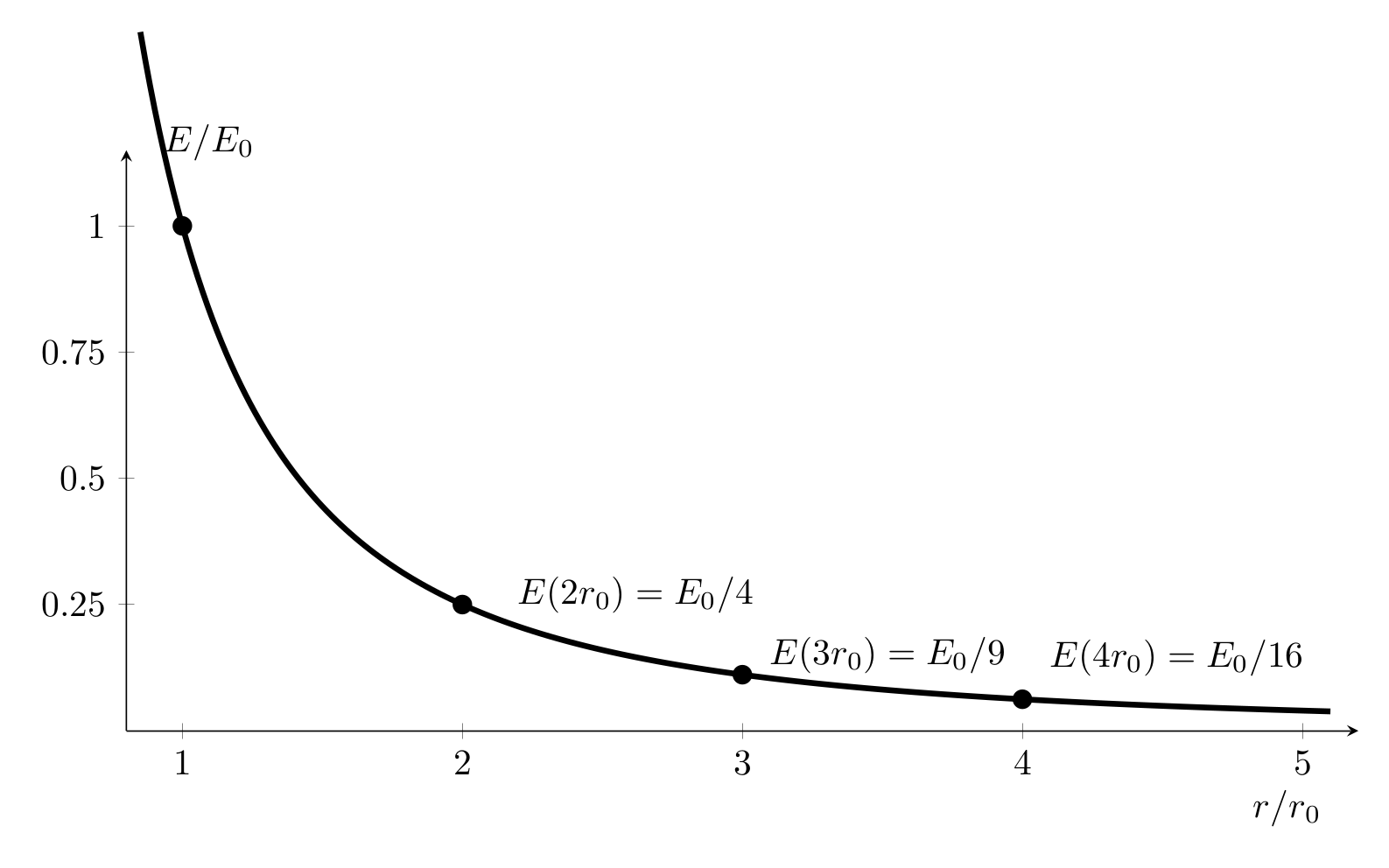
Figure. The field magnitude of an isolated point charge decreases as 1∕r2.
Exercise 11: field versus force
A uniform electric field at a point is
Find the force on each of the following particles:
- a proton, charge +e;
- an electron, charge −e.
Explain why the same field produces opposite force directions.
Exercise 12: write the continuous-source field integral
A volume charge density ρ(r′) occupies a finite source region V ′. Using source coordinate
r′ and observation coordinate r, write the integral expression for the electric field at
r.
Then identify the physical role of each of the following:
No integration is required.
Exercise 13: diagnose conceptual statements
For each statement, decide whether it is correct. If it is incorrect, rewrite it accurately.
- “A negative source charge produces a negative electric-field magnitude.”
- “If the electric field at a point is zero, every individual source field there must also be
zero.”
- “The vector r′ labels the source point and is not a derivative.”
- “A negative test charge experiences force opposite to the electric field.”
- “The point-charge field falls as 1∕r.”
Exercise 14: synthesis - source geometry, field, and force
A source charge
is located at
The observation point is
A test charge
is placed at the observation point.
Find:
- R and R;
- the electric field vector E(r);
- the field magnitude;
- the force vector on the test charge;
- the force magnitude;
- whether the force points toward or away from the source charge.
Part II: Complete Worked Solutions
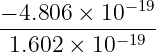
Solution 1: charge quantization
Charge quantization gives
Therefore,
| N | =  | (33)
|
| =  | (34)
|
| ≈−3. | (35) |
Thus the object has three excess electrons:
The negative sign in N = −3 indicates excess negative elementary charges.
Solution 2: Coulomb-force magnitude and sign
The force magnitude is
Substituting,
| F | = (8.99 × 10⁹)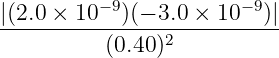 | (38)
|
| ≈ 3.37 × 10⁻⁷ N. | (39) |
Therefore,
Because the charges have opposite signs, the force is attractive.
Solution 3: vector Coulomb force from coordinates
The vector from q1 to q2 is
| R | = r2 − r1 | (41)
|
| = (4 − 1)x + (6 − 2)y | (42)
|
| = 3x + 4y m. | (43) |
Its magnitude is
The unit vector is
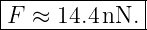
The force magnitude is
| F | = ke | (46)
|
| = (8.99 × 10⁹)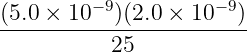 | (47)
|
| ≈ 3.60 × 10⁻⁹ N. | (48) |
Both charges are positive, so the force on q2 points away from q1, in the +R direction.
Hence
| F2←1 | = FR | (49)
|
| ≈ (3.60 × 10⁻⁹)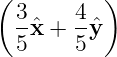 N. N. | (50) |
Thus
Solution 4: source point, observation point, and separation vector
The separation vector is
| R | = r − r′ | (52)
|
| = (5 − 2)x + [3 − (−1)]y + (3 − 3)z | (53)
|
| = 3x + 4y m. | (54) |
Therefore,
Its magnitude is
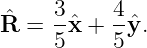
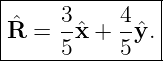
The unit vector is
Solution 5: field magnitude and direction from a negative point charge
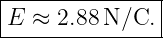
The field magnitude is
| E | = ke | (58)
|
| = (8.99 × 10⁹)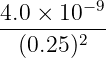 | (59)
|
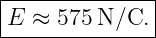
| ≈ 5.75 × 10² N/C. | (60) |
Thus
Because the source charge is negative, the field points radially toward the charge.
Solution 6: force on a negative test charge
Use
Then
| F | = (−6.0 × 10⁻⁹)(250x − 150y) N | (63)
|
| = (−1.50 × 10⁻⁶x + 9.00 × 10⁻⁷y) N. | (64) |
Therefore,
Its magnitude is
| F | =  μN μN | (66)
|
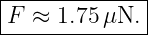
| ≈ 1.75 μN. | (67) |
Hence
The negative sign of qt reverses the force direction relative to E.
Solution 7: cancellation by symmetry
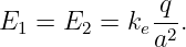
Each charge is a distance a from the origin, so the two field magnitudes are equal:
The field from the left positive charge points toward +x, while the field from the right positive
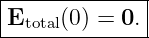
charge points toward −x. Therefore,
Hence
The cancellation occurs because the fields have equal magnitude and opposite direction.
Solution 8: two-dimensional vector superposition
The first field is
The second field has components
| E2x | = 300 cos 120∘ = −150 N/C, | (73)
|
| E2y | = 300 sin 120∘ ≈ 259.8 N/C. | (74) |
Thus
Add the vectors:
| Etotal | = E1 + E2 | (76)
|
| = (250x + 259.8y) N/C. | (77) |
Therefore,
The magnitude is
| Etotal | =  N/C N/C | (79)
|
| ≈ 360.6 N/C. | (80) |
The direction is
| 𝜃 | = tan −1 | (81)
|
| ≈ 46.1∘. | (82) |
Hence
Solution 9: opposite charges and a midpoint field
At the origin, each source is 0.20 m away. The magnitude from either charge is
| Eeach | = ke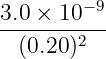 | (84)
|
| ≈ 674 N/C. | (85) |
The positive charge at x = −0.20 m produces a field toward +x at the origin. The negative charge
at x = +0.20 m also produces a field toward +x because the field points toward a negative
charge.
Therefore the two fields add:
Thus
Solution 10: inverse-square scaling
For a point charge,
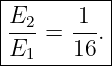
Therefore,
 | =  2 2 | (89)
|
| =  2 2 | (90)
|
| =  . . | (91) |
So
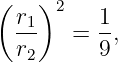
For the second part, require
Then
so
Solution 11: field versus force
For a proton,
Therefore,
| Fp | = qpE | (97)
|
| = (1.602 × 10⁻¹⁹)(500)y N | (98)
|
| ≈ 8.01 × 10⁻¹⁷y N. | (99) |
Thus
For an electron,
Hence
The field is the same in both cases. The force reverses because the particle charges have opposite
signs.
Solution 12: write the continuous-source field integral
The electric field is
The factors have the following meanings:
- ρ(r′) is the charge density at the source point;
- dV ′ is an infinitesimal source volume;
- r − r′ is the vector from the source element to the observation point;
- |r − r′|3 combines with the separation vector so that the magnitude scales as 1∕R2
while retaining direction.
The prime distinguishes the integration/source coordinate from the observation coordinate.
Solution 13: diagnose conceptual statements
- Incorrect. Electric-field magnitude is nonnegative. A negative source charge reverses
the field direction so that the field points toward the source.
- Incorrect. Nonzero individual source fields can cancel vectorially, producing zero total
field.
- Correct. The prime is a source-coordinate label, not differentiation.
- Correct. Since F = qtE, a negative test charge reverses the force direction relative to
E.
- Incorrect. The electrostatic point-charge field magnitude decreases as 1∕r2.
Solution 14: synthesis - source geometry, field, and force
The separation vector is
| R | = r − r′ | (104)
|
| = (4 − 1)x + [2 − (−2)]y | (105)
|
| = 3x + 4y m. | (106) |
Thus
The point-charge field is
Substituting,
| E | = (8.99 × 10⁹)(−8.0 × 10⁻⁹) N/C N/C | (109)
|
| ≈ (−1.73x − 2.30y) N/C. | (110) |
Therefore,
The field magnitude is
The force on the positive test charge is
| F | = qtE | (113)
|
| = (5.0 × 10⁻⁹)(−1.73x − 2.30y) N | (114)
|
| ≈ (−8.63x − 11.5y) × 10−9 N. | (115) |
Thus
Its magnitude is
Because the source charge is negative and the test charge is positive, the force points toward the
source charge.
Common mistakes
- Forgetting charge signs. Use magnitudes for scalar force size, but use signed charge
in vector formulas.
- Using the wrong separation vector. For a source at r′ and observation point r,
use R = r − r′.
- Adding field magnitudes instead of vectors. Superposition is componentwise
vector addition.
- Confusing field direction with force direction. A negative test charge experiences
force opposite to E.
- Using 1∕r instead of 1∕r2. The electrostatic point-charge field is inverse square.
- Treating r′ as a derivative. The prime is only a source-coordinate label.
What EM05E reinforces
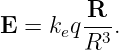
The essential field relation is
It combines source strength, source-to-observation geometry, inverse-square magnitude, and vector
direction in one expression.
For many sources,
and for a continuous charge distribution the sum becomes an integral over source points.
These ideas prepare the next article, EM06, where electric flux and oriented area vectors will be
introduced before Gauss’s Law.
References
[1] David J. Griffiths, Introduction to Electrodynamics, 4th ed., Cambridge University
Press, 2017.
[2] Samuel J. Ling, Jeff Sanny, and William Moebs, University Physics, Volume 2,
OpenStax, 2016, chapters on electric charge, electric field, and Gauss’s law.
[3] Edward M. Purcell and David J. Morin, Electricity and Magnetism, 3rd ed.,
Cambridge University Press, 2013.
[4] Richard P. Feynman, Robert B. Leighton, and Matthew Sands, The Feynman Lectures
on Physics, Volume II, Addison-Wesley, 1964, chapters on electrostatics and the electric
field.
[5] Massachusetts Institute of Technology, 8.02 Physics II: Electricity and Magnetism,
MIT OpenCourseWare, materials on Coulomb’s law and electric fields.

![[parent]](https://images.physicslibrary.org/images/uparrow.png)