Electromagnetic Waves, Antennas, and RF: Electric Charge and the Electric Field

Electromagnetic Waves, Antennas, and RF:
Electric Charge and the Electric Field

EM01–EM04 built the mathematical language needed to describe fields in space and time. EM05 now introduces the first specifically electromagnetic field: the electric field.

The starting physical quantity is Electric Charge. Charges exert forces on one another. Instead of describing those forces only as direct interactions between pairs of particles, Electromagnetism assigns an electric field to space. A source charge creates a field, and another charge responds to the field at its location.

This change in viewpoint is essential for everything that follows. Later articles will allow the electric field to vary in time, couple it to the magnetic field through Maxwell’s equations, and show that electromagnetic disturbances propagate as radio waves. For now, the fields are electrostatic and the source charges are treated as stationary [1, 2, 3].

1 Electric charge

Electric charge is a property of matter that determines how strongly an object participates in electromagnetic interactions. The SI unit of charge is the coulomb:

|--------| -[q-] =-C.|

(1)

Charge comes in two signs, conventionally called positive and negative. The elementary charge magnitude is

|--------------−19---| -e ≈-1.602 ×-10---C.--

(2)

A proton has charge +e and an electron has charge −e.

1.1 Charge is quantized

For ordinary isolated particles and collections of particles, net charge appears in integer multiples of the elementary charge:

|--------| -q =-N-e,-

(3)

where N is an integer. At macroscopic scales the elementary step is so small that charge is often modeled as a continuous quantity.

1.2 Charge is conserved

In an isolated system, total electric charge is conserved. Charge may move from one body to another, but the net amount does not simply appear or disappear in classical electromagnetic processes.

This conservation law will later become part of the mathematical consistency of Maxwell’s equations.

2 Like charges repel and unlike charges attract

Experiments show a simple sign rule:

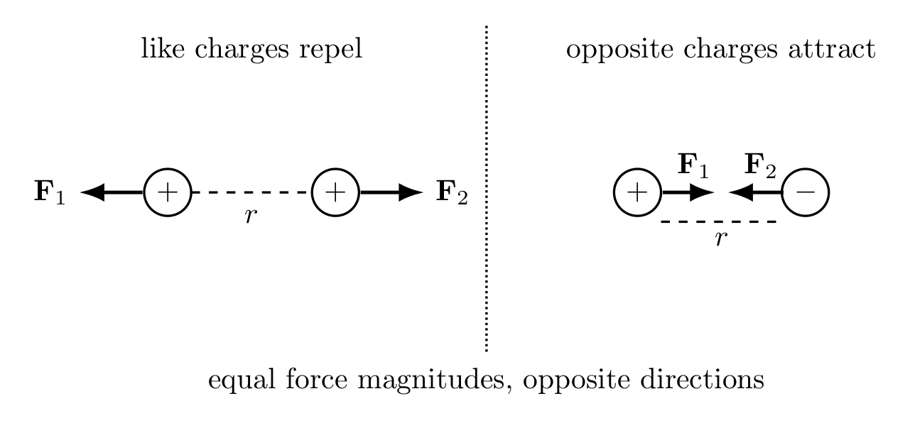
|------------------------------------------| -like-signs-repel,----opposite-signs-attract.|

(4)

Figure. Like charges repel and unlike charges attract. The forces on the two charges have equal magnitude and opposite direction.

The sign rule gives the direction of the force. Coulomb’s law gives its magnitude.

3 Coulomb’s law: magnitude

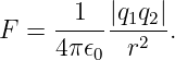
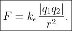
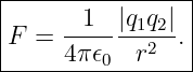
Consider two stationary point charges q₁ and q₂ separated by a distance r. The magnitude of the electrostatic force between them is

|----------------| | 1 |q1q2| | |F = -------2--.| ------4π𝜖0--r----

(5)

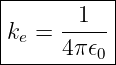
The constant

𝜖0

(6)

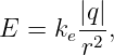
is the vacuum permittivity. It is common to define Coulomb’s constant

|----------| | --1--| |ke = 4π𝜖 | ---------0--

(7)

so that

|-------------| F = ke|q1q2|. | ---------r2----

(8)

Numerically,

k ≈ 8.99 × 109 N m2 ∕C2. e

(9)

3.1 The inverse-square dependence

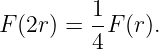
The factor

1- r2

(10)

means that doubling the separation reduces the force magnitude by a factor of four:

1 F (2r) = -F (r). 4

(11)

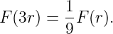
Tripling the separation reduces the force by a factor of nine:

1 F (3r) = 9F (r).

(12)

This inverse-square structure will later reappear when electromagnetic power spreads over larger spherical surfaces.

4 Coulomb’s law as a vector equation

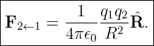
The magnitude-only formula does not record direction. To write Coulomb’s law as a vector equation, define the vector from source charge q₁ to observation charge q₂ as

R = r2 − r1.

(13)

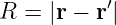
Its magnitude is

R = |R |,

(14)

and its unit direction is

R ˆR = --. R

(15)

The force on q₂ due to q₁ is then

|--------------------| |F2←1 = --1--q1q2ˆR. | ---------4π-𝜖0-R2-----|

(16)

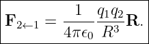
An equivalent form is

|--------------------| | 1 q1q2 | |F2←1 = -------3-R. | ---------4π-𝜖0-R------

(17)

The signed product q₁q₂ automatically handles attraction or repulsion.

5 Source point and observation point

The previous notation becomes especially useful when we separate the location of the source from the location where a field is evaluated.

Let the source charge lie at

′ r

(18)

and let the observation point be

r.

(19)

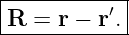
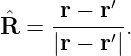
Define the separation vector

|----------′-| -R--=-r-−-r.-|

(20)

Then

′ R = |r − r |

(21)

and

r − r′ Rˆ = ------′. |r − r|

(22)

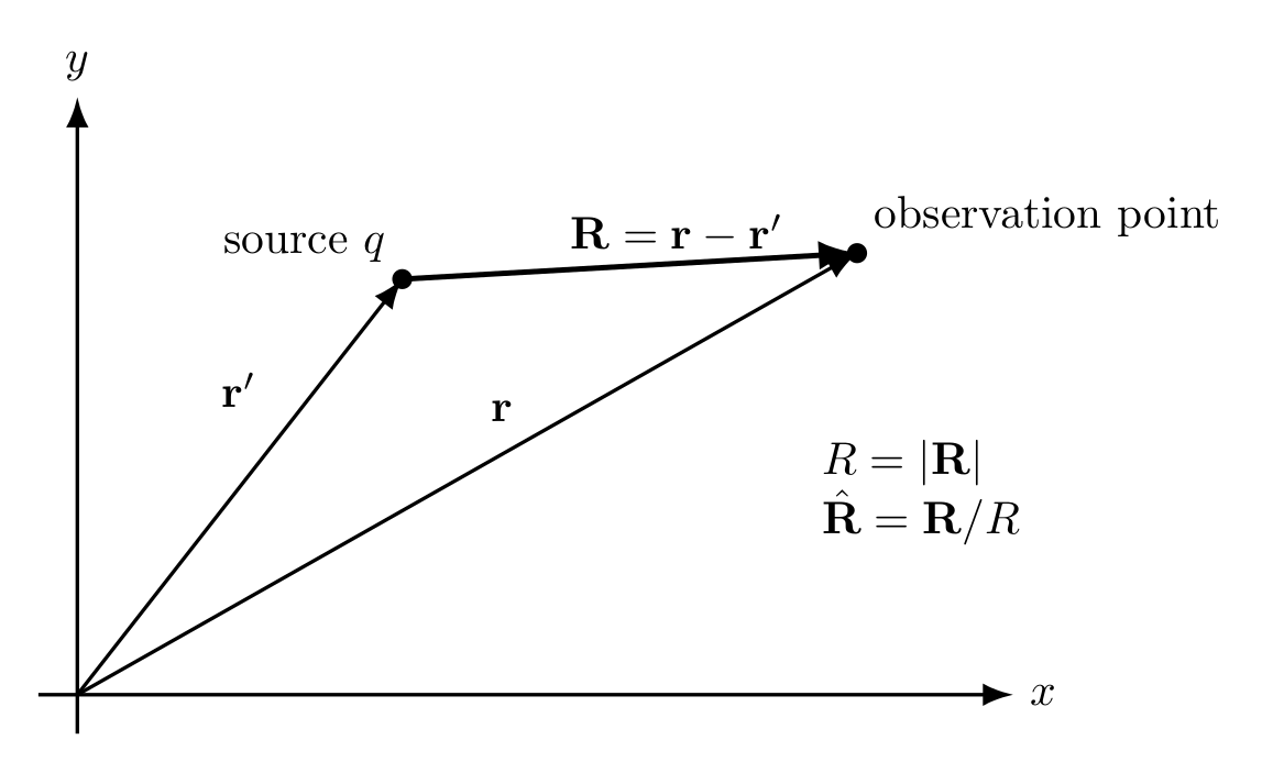
Figure. The source point r′ and observation point r are connected by the separation vector R = r − r′. This geometry will later be reused for continuous charge distributions, retarded fields, antenna apertures, and radiation integrals.

The prime on r′ is not a derivative. It is simply a label distinguishing the source coordinate from the observation coordinate.

6 From force to field

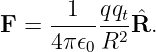
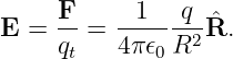
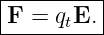
Suppose a source configuration is fixed in space. Place a small positive test charge q_t at an observation point. If the force on the test charge is F, define the electric field by

|--------| | F- | |E = qt.| ---------

(23)

Equivalently,

|--------| F--=-qtE.-

(24)

The electric field describes the force per unit positive charge that would act at a point.

6.1 Units of electric field

From the definition,

N [E ] =--. C

(25)

Thus

|------------| |[E] = N/C. | -------------

(26)

Later we will also encounter the equivalent unit volts per meter.

6.2 Why the test charge is conceptually small

The test charge is imagined to be small enough that it does not significantly disturb the source configuration whose field we are trying to characterize. The electric field is therefore attributed to the source, not to the particular probe used to measure it.

7 Electric field of a point charge

For a point source charge q located at r′, Coulomb’s law gives the force on a test charge q_t at r:

F = -1---qqtˆR. 4π𝜖0 R2

(27)

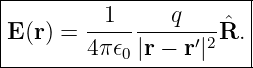
Divide by q_t:

F 1 q E = -- = ------2Rˆ. qt 4π𝜖0R

(28)

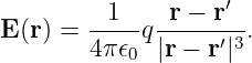
Therefore,

|-----------------------| | -1------q----ˆ | E (r) = 4π𝜖0 |r − r′|2R. | -------------------------

(29)

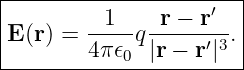
Using R∕R³ instead of R∕R²,

|----------------------| | 1 r − r′ | |E(r) = -----q--------.| --------4π-𝜖0-|r −-r′|3--

(30)

This formula contains both magnitude and direction.

8 Direction of the point-charge field

If q > 0, the electric field points radially away from the source charge. If q < 0, the field points radially toward the source charge.

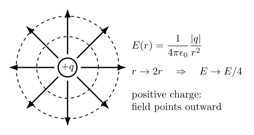
Figure. A positive point charge produces a radial field directed outward. The field magnitude decreases as 1∕r². Reversing the sign of the source charge reverses every field vector.

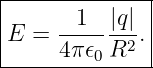
The magnitude is

|--------------| | 1 |q| | |E = --------.| ------4π𝜖0-R2--

(31)

Notice that the electric field exists as a function of position even before a second charge is introduced. A probe charge merely experiences the field through

F = q E. t

(32)

9 Worked example 1: electric field magnitude from a point charge

A charge

q = +2.0 nC

(33)

is located at the origin. Find the electric field magnitude at a point 0.30 m away.

Using

E = k |q|, e r2

(34)

we obtain

E	= (8.99 × 10⁹)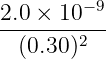 N/C	(35)
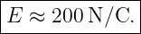
	≈ 2.00 × 10² N/C.	(36)

Thus

|--------------| -E-≈--200N/C.--|

(37)

Because the source charge is positive, the field points radially outward.

10 Worked example 2: force on a charge placed in a known field

Suppose

E = (300 ˆx − 100ˆy )N/C

(38)

and a charge

qt = − 4.0nC

(39)

is placed at that point.

The force is

F = q E. t

(40)

Therefore,

F	= (−4.0 × 10⁻⁹)(300x − 100y) N	(41)
	= (−1.20 × 10⁻⁶x + 4.0 × 10⁻⁷y) N.	(42)

Hence

|--------------------------| |F = (− 1.20ˆx + 0.40ˆy )μN. | ---------------------------

(43)

Because the test charge is negative, the force points opposite the electric-field direction.

11 Superposition of electric fields

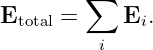
Electrostatic fields obey the principle of superposition. If several source charges are present, the total field is the vector sum of the individual fields:

|----------------------------| -Etotal =-E1-+-E2-+-⋅⋅⋅-+-EN-.-

(44)

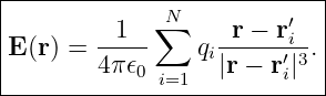
For point charges q_i at positions r_i′, the total field at observation point r is

|---------------------------| | 1 ∑N r − r′ | E (r) = ----- qi-----i′3. | | 4π𝜖0 i=1 |r − ri| | -----------------------------

(45)

Each source contributes independently, and the resulting vectors are added component by component.

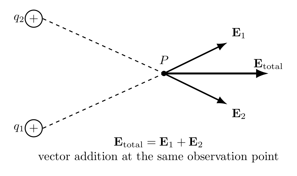
Figure. Two source charges contribute fields E₁ and E₂ at the same observation point. The total electric field is their vector sum.

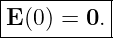
12 Worked example 3: two equal positive charges on an axis

Two equal positive charges are placed symmetrically at

x = − a and x = +a.

(46)

At the origin, the field from the left charge points in the +x direction, while the field from the right charge points in the −x direction. The magnitudes are equal.

Therefore,

|----------| |E (0 ) = 0.| -----------

(47)

This is a useful reminder that electric fields are vectors: nonzero individual contributions can cancel exactly.

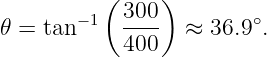
13 Worked example 4: two-dimensional superposition

Suppose at a point P two source charges produce

E1 = 400ˆx N/C

(48)

and

E2 = 300 ˆyN/C.

(49)

Then

E = 400ˆx + 300 ˆyN/C. total

(50)

Its magnitude is

E_total	= N/C	(51)
	= 500 N/C.	(52)

Thus

|-----------------| Etotal =-500-N/C.--

(53)

The direction above the +x axis is

( ) −1 300- ∘ 𝜃 = tan 400 ≈ 36.9 .

(54)

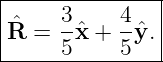
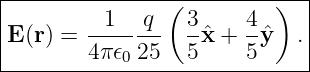
14 Worked example 5: point charge at a nonzero source location

A charge q is located at

r′ = 1ˆx + 2ˆy m.

(55)

Find the separation vector to the observation point

r = 4xˆ+ 6ˆym.

(56)

The separation vector is

R	= r − r′	(57)
	= (4 − 1)x + (6 − 2)y m	(58)
	= 3x + 4y m.	(59)

Its magnitude is

√ ------- R = 32 + 42 = 5m.

(60)

The unit vector is

|--------------| | 3 4 | |ˆR = -ˆx + --ˆy.| ------5----5----

(61)

Therefore the point-charge field at r can immediately be written as

|---------------(---------)--| E (r) = --1--q-- 3ˆx + 4-ˆy .| --------4π-𝜖025---5----5------

(62)

15 Worked example 6: scaling with distance

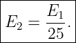
Suppose the electric-field magnitude from a point charge is

E1

(63)

at distance r₁. At distance

r2 = 5r1,

(64)

inverse-square scaling gives

	= ²	(65)
	= ²	(66)
	= .	(67)

Therefore,

|----------| | E1- | |E2 = 25 .| -----------

(68)

16 From point charges to continuous charge distributions

Macroscopic objects contain enormous numbers of charged particles. Rather than summing over every microscopic charge, it is often useful to define a continuous charge density.

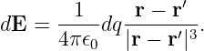
For a volume charge density ρ(r′), an infinitesimal source volume dV ′ contains charge

′ ′ dq = ρ(r) dV .

(69)

Its infinitesimal field contribution at observation point r is

--1-- -r-−-r′- dE = 4π𝜖0dq |r − r′|3.

(70)

Substituting dq = ρ(r′)dV ′ gives

1 r − r′ dE = -----ρ(r′)------′3dV ′. 4π 𝜖0 |r − r|

(71)

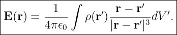
Integrating over the source volume gives

|------------∫-------------------| | 1 ′ r − r′ ′ | |E(r) = 4π-𝜖- ρ(r )|r-−-r′|3dV .| ------------0---------------------

(72)

This integral is only a preview here. EM06 and later articles will develop flux, Gauss’s Law, and continuous source distributions more systematically.

The important structural pattern is already visible:

|---------------------------∫---------------------------------------------| | | field at observation point = source contribution from each source point. | ---------------------------------------------------------------------------

(73)

That same source-to-observation geometry will return much later when antenna apertures are treated as many small radiating source elements.

17 Electric field lines as a visualization tool

Electric field lines are graphical aids. They are drawn so that the tangent to a field line gives the local direction of E.

For a positive isolated point charge, the lines point radially outward. For a negative charge, they point radially inward.

Field lines are not physical strings or trajectories carried through space. They are a way of visualizing a vector field.

18 Field versus force

It is important to keep two quantities distinct:

|--------------------------------------------| E describes the field created by the sources, ----------------------------------------------

(74)

whereas

|--------------------------------------------------| F = qE describes the force on a particular charge. ----------------------------------------------------

(75)

The same field can exert different forces on different charges because the response depends on the test charge q.

A negative charge experiences a force opposite to E. This does not mean the electric field itself has reversed.

19 Common mistakes

19.1 Using 1∕r instead of 1∕r²

The electrostatic point-charge field magnitude decreases as

1 E ∝ -2, r

(76)

not as 1∕r.

19.2 Dropping the direction

Coulomb’s law and electric field are fundamentally vector relations. A magnitude alone is incomplete when more than one source is present.

19.3 Confusing source position and observation position

The field is evaluated at r, but the source lies at r′. The relevant separation is

′ R = r − r.

(77)

19.4 Assuming a negative charge means a negative field magnitude

The magnitude E is nonnegative. The sign of the source charge determines the field direction.

19.5 Confusing electric field with force

The field exists independently of the particular test charge. The force depends on both the field and the test charge:

F = qtE.

(78)

20 Why EM05 matters for radio waves

Radio waves are not electrostatic fields, but the electric field in a radio wave is the same physical field quantity introduced here. Later the source charges and currents will vary in time, and Maxwell’s equations will couple the electric and magnetic fields.

The progression is therefore

|---------------------------------------------------------------------------------| charge → E → time -varying fields → Maxwell equations → electromagnetic waves. | ----------------------------------------------------------------------------------

(79)

For antennas, another important progression will be

|----------------------------∫--------------------------| | | distributed sources → dE → dE → radiation pattern. | ---------------------------------------------------------

(80)

EM05 supplies the source/observation geometry and superposition language needed for that later development.

Summary

The essential results of EM05 are:

Electric charge is measured in coulombs and occurs with positive or negative sign.
Charge is conserved and appears in elementary units of magnitude e.
Coulomb’s law for two stationary point charges has inverse-square magnitude:
$1 |q1q2| F = 4π𝜖---r2--. 0$
The electric field is force per unit positive test charge:
$F- E = qt.$
A point charge produces
$1 r − r′ E(r) = -----q--------. 4π 𝜖0 |r − r′|3$
Positive source charges produce outward radial fields; negative source charges produce inward radial fields.
Electric fields superpose linearly:
$∑ Etotal = Ei. i$
Source-point notation r′ and observation-point notation r will become increasingly important in continuous-source and antenna calculations.

The next lesson, EM06, introduces electric flux and the oriented area vector dA. That will prepare the geometric machinery needed for Gauss’s law.

References

[1] David J. Griffiths, Introduction to Electrodynamics, 4th ed., Cambridge University Press, 2017.

[2] Samuel J. Ling, Jeff Sanny, and William Moebs, University Physics, Volume 2, OpenStax, 2016, chapters on electric charge, electric field, and Gauss’s law.

[3] Edward M. Purcell and David J. Morin, Electricity and Magnetism, 3rd ed., Cambridge University Press, 2013.

[4] Richard P. Feynman, Robert B. Leighton, and Matthew Sands, The Feynman Lectures on Physics, Volume II, Addison-Wesley, 1964, chapters on electrostatics and the electric field.

[5] Massachusetts Institute of Technology, 8.02 Physics II: Electricity and Magnetism, MIT OpenCourseWare, materials on Coulomb’s law and electric fields.

"Antennas Electromagnetic Waves" is owned by bloftin.
(view preamble)