1 Where GPSORB04 fits in the derivation chain
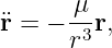
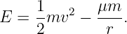
The starting point remains the ideal two-body equation derived in GPSORB01,
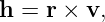
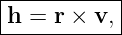
and the conserved specific angular momentum developed in GPSORB03,
Because  is constant, the motion is confined to a fixed plane perpendicular to
  . What
remains is to determine the shape of the trajectory within that plane.
. What
remains is to determine the shape of the trajectory within that plane.
The development in this article is
The central idea is that the orbit equation is not imposed geometrically. It is extracted from
Newton’s differential equation through its conserved quantities.
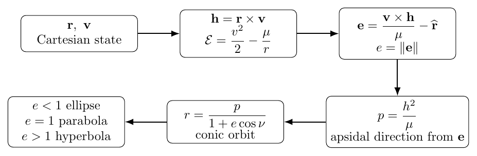
Figure 1. The Cartesian state determines conserved quantities, which in turn determine the conic
orbit and its classification.
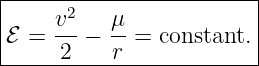
2 Specific mechanical energy
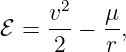
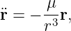
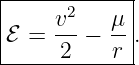
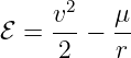
For a satellite of mass  , the ordinary mechanical energy is
Orbital mechanics usually divides by the satellite mass and works with specific mechanical
energy,
The units are
The first term is specific kinetic energy and the second is gravitational potential energy per unit
mass, with zero potential chosen at infinite distance.
2.1 Derivation directly from the equation of motion
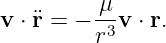
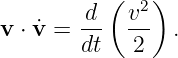
Take the dot product of Eq. (1) with the velocity  :
:
The left-hand side is
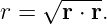
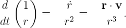
For the right-hand side, begin with
Differentiation gives
Therefore
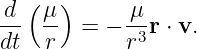
Multiplying by  ,
,
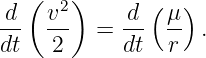
Equation (5) therefore becomes
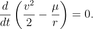
Move both terms to the same side:
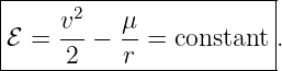
Hence
This is the energy first integral of the Kepler problem.
2.2 Physical interpretation
As a satellite falls inward,  decreases and the potential term
  becomes more negative.
Since the sum
becomes more negative.
Since the sum  remains constant, the kinetic term
  must increase. As the satellite climbs
outward, the reverse occurs.
must increase. As the satellite climbs
outward, the reverse occurs.
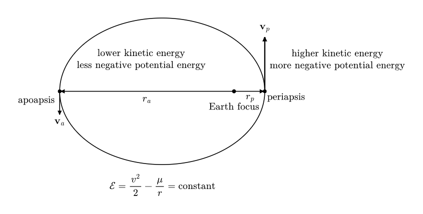
Figure 2. In an elliptical orbit the satellite moves fastest at periapsis and slowest at apoapsis
while total specific mechanical energy remains constant.
This energy exchange is another way to understand why the orbital speed is not generally constant
even though no dissipative force is present.
3 Why angular momentum alone is not enough
The conserved vector  determines the orbital plane and the amount of transverse motion, but it
does not by itself determine the orientation of the ellipse within that plane. Two ellipses can lie in
the same plane and have the same angular-momentum magnitude while pointing their periapsides
in different directions.
determines the orbital plane and the amount of transverse motion, but it
does not by itself determine the orientation of the ellipse within that plane. Two ellipses can lie in
the same plane and have the same angular-momentum magnitude while pointing their periapsides
in different directions.
A second conserved vector is therefore needed. The inverse-square gravitational field has a special
additional invariant known as the eccentricity vector. In classical mechanics it is closely related to
the Laplace-Runge-Lenz vector.
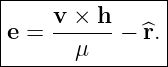
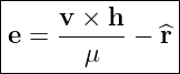
4 The eccentricity vector
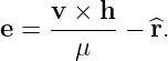
Define
where
The eccentricity vector is dimensionless. Its magnitude is the orbital eccentricity,
For a noncircular Keplerian orbit,  points from the attracting focus toward periapsis.
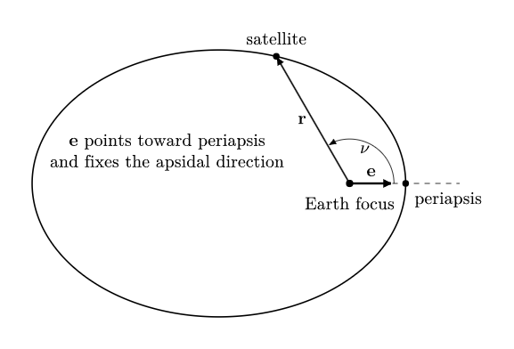
Figure 3. The eccentricity vector points toward periapsis, and the true anomaly is measured from
that direction to the position vector.
5 Proving that the eccentricity vector is constant
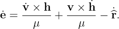
The constancy of  is special to the inverse-square gravitational law. Differentiate
Eq. (14):
is special to the inverse-square gravitational law. Differentiate
Eq. (14):
Because  ,
,
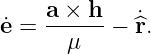
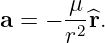
The two-body acceleration is
Hence
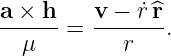
Use the vector triple-product identity
With  ,
,  , and
, and  ,
,
Now
so
Substituting into Eq. (20),
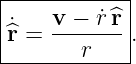
But differentiating  gives
gives
Therefore the two terms in Eq. (18) cancel exactly:
Thus the eccentricity vector is constant in both magnitude and direction for the ideal Kepler
problem.
6 The geometric meaning of the eccentricity vector
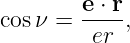
Because  is fixed in the orbital plane, it provides a natural reference direction. Define
the true anomaly
is fixed in the orbital plane, it provides a natural reference direction. Define
the true anomaly  as the angle from
  to the instantaneous position vector
  .
Then
.
Then
This apparently simple dot product is the key to deriving the conic equation.
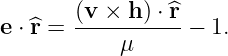
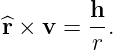
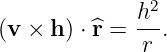
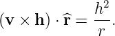
First use Eq. (14):
The scalar triple product may be cyclically permuted:
Since
we have
Therefore
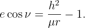
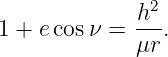
Substitution into Eq. (29) gives
Rearrange:
Hence
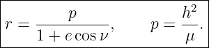
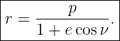
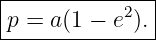
Define the semilatus rectum
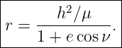
The orbit equation becomes
This is the polar equation of a conic section with the attracting body at one focus.
7 Why this is a major result
Equation (38) was obtained entirely from the Newtonian equation of motion. No ellipse was
assumed. The derivation shows that inverse-square gravity forces the trajectory to be a conic
section.
The constants have direct physical meanings:
| Quantity | Physical role |
| 
| fixes the orbital plane and transverse angular momentum per
unit mass |
| 
| sets the semilatus rectum through  |
| 
| fixes the periapsis direction in the orbital plane |
| 
| determines the conic shape |
| 
| locates the satellite around the conic relative to periapsis |
8 Conic classification from eccentricity
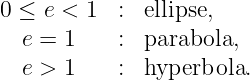
The same orbit equation describes all nondegenerate Keplerian conics:
The special case  is a circle. In that case the eccentricity vector vanishes and there is no
unique periapsis direction.
is a circle. In that case the eccentricity vector vanishes and there is no
unique periapsis direction.
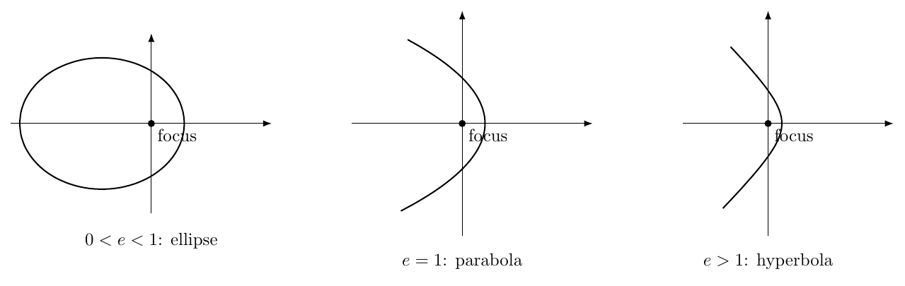
Figure 4. The same focus-centered orbit equation produces elliptical, parabolic, and hyperbolic
trajectories as eccentricity crosses unity.
The conic classification emerges even more deeply from energy, as shown next.
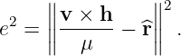
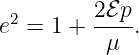
9 The relation among energy, angular momentum, and eccentricity
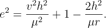
Square the magnitude of Eq. (14):
Expanding,
Because  lies in the orbital plane and
  is normal to it,
so
From Eq. (33),
Thus
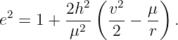
Factor  :
:
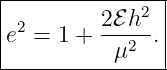
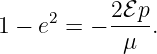
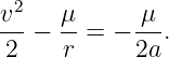
Recognizing the specific mechanical energy,
This equation is one of the most useful bridges between orbital dynamics and conic
geometry.
Because  and
and  , the sign of
  determines whether
  is less than, equal to, or
greater than one:
is less than, equal to, or
greater than one:
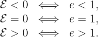
Therefore negative specific orbital energy corresponds to a bound ellipse, zero energy to the
parabolic escape boundary, and positive energy to an unbound hyperbola.
10 Periapsis and apoapsis from the conic equation
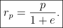
Periapsis occurs at  , so
, so  . Equation (38) gives
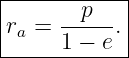
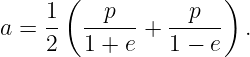
For an ellipse, apoapsis occurs at  , so
, so  :
:
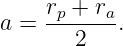
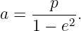
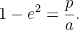
The semimajor axis of an ellipse is half the sum of the apsidal distances,
Substituting Eqs. (49) and (50),
Combining the fractions,
Hence
This relation applies to ellipses and, with signed semimajor-axis conventions, extends naturally to
hyperbolic conics.
11 Energy and semimajor axis
Substitute
into Eq. (47):
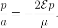
Rearrange:
For an ellipse, Eq. (54) gives
Therefore
Cancel the nonzero  :
:
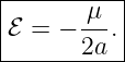
This is a remarkably compact result: for every ideal elliptical orbit having the same semimajor
axis, the total specific mechanical energy is the same, regardless of eccentricity.
12 The vis-viva equation
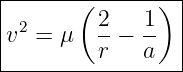
Combine the energy definition
with Eq. (60):
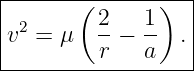
Multiply by two and solve for  :
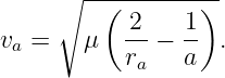
:
This is the vis-viva equation. It gives the speed at any orbital radius without first solving the full
time history of the trajectory.
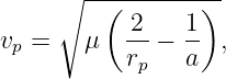
At periapsis,
and at apoapsis,
For an ellipse,  , so
, so  , consistent with both energy conservation and Kepler’s
second law.
, consistent with both energy conservation and Kepler’s
second law.
13 Radial and transverse velocity components
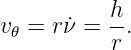
GPSORB03 established
when the polar angle is measured in the orbital plane from a fixed apsidal direction. Therefore the
transverse speed is
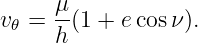
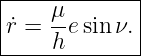
Using Eq. (38),
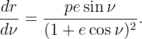
Differentiate the orbit equation with respect to  :
:
Since
and
substitution gives
Thus the in-plane velocity may be written as
This form is useful later when converting between orbital elements and Cartesian state
vectors.
14 A numerical GPS-like example
Consider an idealized medium-Earth orbit with
Use
The periapsis and apoapsis radii are
The specific mechanical energy is
The semilatus rectum is
The specific angular-momentum magnitude is
Using vis-viva,
Even for a small eccentricity of only  , the speed changes measurably over the
orbit.
, the speed changes measurably over the
orbit.
15 From a Cartesian state directly to the conic
Given one inertial state  , the ideal conic can be reconstructed without numerically
integrating the trajectory first.
, the ideal conic can be reconstructed without numerically
integrating the trajectory first.
Compute
and
Then
For a bound noncircular orbit,
The true anomaly can be found robustly with an atan2 construction. One convenient form
is
with the sign of  obtained from the radial velocity or from a triple product involving
  .
This avoids quadrant ambiguity that appears if only an inverse cosine is used.
.
This avoids quadrant ambiguity that appears if only an inverse cosine is used.
16 Connection to the GPS broadcast ephemeris
The legacy GPS navigation message does not transmit an instantaneous Cartesian state vector.
Instead, among its broadcast ephemeris parameters it provides the eccentricity  and the square
root of semimajor axis
and the square
root of semimajor axis  , together with angular elements, rates, an epoch, and harmonic
correction coefficients. The official interface specification describes these parameters as Keplerian in
appearance while noting that their values are obtained by fitting a propagated satellite trajectory
over a finite interval.
, together with angular elements, rates, an epoch, and harmonic
correction coefficients. The official interface specification describes these parameters as Keplerian in
appearance while noting that their values are obtained by fitting a propagated satellite trajectory
over a finite interval.
The results derived in this article explain why  and
and  are such natural coordinates for the
broadcast model:
are such natural coordinates for the
broadcast model:
so  controls the orbital energy and characteristic size while
  controls the departure from
circularity and the apsidal geometry. Later articles will show how
controls the departure from
circularity and the apsidal geometry. Later articles will show how  is converted
to
is converted
to  , then to mean motion, mean anomaly, eccentric anomaly, and finally satellite
position.
, then to mean motion, mean anomaly, eccentric anomaly, and finally satellite
position.
17 Important limiting cases and cautions
17.1 Circular orbit
For  ,
,
so the eccentricity-vector direction is undefined. The orbit is still perfectly well defined,
but periapsis has no unique direction because every point on a circle is geometrically
equivalent.
17.2 Radial motion
If  , then the motion is purely radial and the standard nondegenerate conic-element
description breaks down. This is a singular limiting case, not the normal satellite-orbit
situation.
, then the motion is purely radial and the standard nondegenerate conic-element
description breaks down. This is a singular limiting case, not the normal satellite-orbit
situation.
17.3 Perturbed motion
For a real GPS satellite, Earth’s nonspherical gravity, third-body forces, solar radiation pressure,
and other perturbations cause the ideal invariants to evolve slowly. In that setting one can still
define instantaneous or osculating values of  ,
,  , and
, and  , but they are no longer exactly
constant.
, but they are no longer exactly
constant.
This distinction matters later when interpreting broadcast ephemeris parameters: the equations
look Keplerian, but the transmitted coefficients represent a finite-interval fit to a perturbed orbit
rather than a set of eternal two-body constants.
18 Summary of the derivation
Starting from Newton’s inverse-square two-body equation,
we obtained a second scalar first integral,
Together with the conserved angular momentum,
the inverse-square law admits the conserved eccentricity vector,
Its dot product with  yields
For an ellipse,
Finally,
provides the vis-viva speed relation.
The next step is to use  ,
,  , and the inertial reference axes to construct the classical orbital
elements
, and the inertial reference axes to construct the classical orbital
elements  explicitly from a Cartesian state vector.
References
[1] E. D. Kaplan and C. J. Hegarty, eds., Understanding GPS/GNSS: Principles and
Applications, 3rd ed., Artech House, 2017.
[2] R. R. Bate, D. D. Mueller, and J. E. White, Fundamentals of Astrodynamics, Dover
Publications, 1971.
[3] D. A. Vallado, Fundamentals of Astrodynamics and Applications, 4th ed., Microcosm
Press, 2013.
[4] H. D. Curtis, Orbital Mechanics for Engineering Students, 4th ed., Elsevier, 2020.
[5] Global Positioning Systems Directorate, IS-GPS-200N: Navstar GPS Space
Segment/Navigation User Interfaces, 1 August 2022. Available from GPS.gov.



![2
[ℰ] = m--= -J-.
s2 kg](https://images.physicslibrary.org/cache/objects/1260/make4ht/SpecificMechanicalEnergyTheEccentricityVectorAndTheConicOrbitEquation8x.png)



![a × h 1
------= − -2 [^r × (r × v)].
μ r](https://images.physicslibrary.org/cache/objects/1260/make4ht/SpecificMechanicalEnergyTheEccentricityVectorAndTheConicOrbitEquation34x.png)
















![|----------------------------------|
|v = μ-[esinν er + (1 + ecosν )e𝜃].|
-----h------------------------------](https://images.physicslibrary.org/cache/objects/1260/make4ht/SpecificMechanicalEnergyTheEccentricityVectorAndTheConicOrbitEquation118x.png)