Physics Library
 An open source physics library
Encyclopedia | Forums | Docs | Random | Template Test |  
Login
create new user
Username:
Password:
forget your password?
Main Menu
Sections

Meta

Talkback

Downloads

Information
numerical quaternion propagation and IMU attitude state integration (Topic)

Numerical Quaternion Propagation and IMU Attitude State Integration

A gyroscope does not directly measure attitude. It measures angular motion. An inertial navigation or attitude system must integrate that angular motion over time to update an orientation state.

Quaternions are particularly well suited to this task because a unit quaternion can be updated by a finite incremental rotation without introducing an Euler Angle singularity.

This article develops numerical propagation for the PhysicsLibrary passive attitude quaternion

$\displaystyle q = {}^{B}q_I,$ (1)

which maps coordinates from an inertial or reference frame $I$ into a body frame $B$.

For body resolved angular velocity,

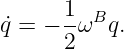
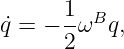
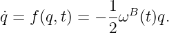
$\displaystyle \dot q = -\frac12 \omega^B q.$ (2)

Over one sample interval, the exact constant rate update is

$\displaystyle q_{k+1} = \delta q_B q_k,$ (3)

where

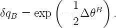
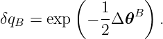
$\displaystyle \delta q_B = \exp \left( -\frac12 \Delta\theta^B \right).$ (4)

Thus the numerical implementation must preserve three convention facts:

  1. the body frame increment has a negative quaternion vector part;
  2. the body resolved increment multiplies on the left;
  3. the propagated quaternion maps reference coordinates into body coordinates.

Convention declaration

PhysicsLibrary uses Hamilton multiplication,

$\displaystyle \mathbf i\mathbf j=\mathbf k, \qquad \mathbf j\mathbf k=\mathbf i, \qquad \mathbf k\mathbf i=\mathbf j, $

with reversed products changing sign.

Quaternion components are displayed scalar first:

$\displaystyle q = q_w+q_x\mathbf i+q_y\mathbf j+q_z\mathbf k.$ (5)

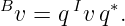
The passive vector transformation is

$\displaystyle {}^{B}v = q\,{}^{I}v\,q^*.$ (6)

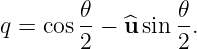
For a positive frame rotation through angle $\theta$ about unit axis $\widehat{\mathbf u}$,

$\displaystyle q = \cos\frac{\theta}{2} - \widehat{\mathbf u} \sin\frac{\theta}{2}.$ (7)

The corresponding DCM satisfies

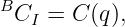
$\displaystyle {}^{B}\mathbf v = {}^{B}C_I\,{}^{I}\mathbf v, \qquad {}^{B}C_I=C(q).$ (8)

From gyroscope measurement to corrected angular rate

A practical body mounted gyroscope measurement can be modeled as

$\displaystyle \boldsymbol\omega_m^B = {}^{B}\boldsymbol\omega_{B/I} + \mathbf b_g + \mathbf n_g,$ (9)

where

$\displaystyle \mathbf b_g $

is gyroscope bias and

$\displaystyle \mathbf n_g $

represents measurement noise.

Given a current bias estimate $\widehat{\mathbf b}_g$, form

$\displaystyle \widehat{\boldsymbol\omega}^B = \boldsymbol\omega_m^B - \widehat{\mathbf b}_g.$ (10)

For a simple zero order hold over sample interval $\Delta t$, the corresponding body resolved delta angle is

$\displaystyle \Delta\boldsymbol\theta^B = \widehat{\boldsymbol\omega}^B \Delta t.$ (11)

If the IMU itself supplies a delta angle measurement, that integrated quantity should normally be used directly after the appropriate bias correction and manufacturer specified compensation rather than unnecessarily converting it to a rate and integrating it again.

Exact exponential increment

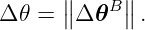
Let

$\displaystyle \Delta\theta = \left\lVert \Delta\boldsymbol\theta^B \right\rVert.$ (12)

If

$\displaystyle \Delta\theta\neq0, $

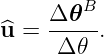
define the unit increment axis

$\displaystyle \widehat{\mathbf u} = \frac{ \Delta\boldsymbol\theta^B }{ \Delta\theta }.$ (13)

The exact passive body increment is

$\displaystyle \delta q_B = \cos\frac{\Delta\theta}{2} - \widehat{\mathbf u} \sin\frac{\Delta\theta}{2}.$ (14)

Equivalently,

$\displaystyle \delta q_B = \exp \left( -\frac12 \Delta\boldsymbol\theta^B \right).$ (15)

In scalar first array notation,

$\displaystyle \delta\mathbf q_B = \begin{bmatrix} \cos(\Delta\theta/2) \ -\df... ...\sin(\Delta\theta/2) }{ \Delta\theta } \Delta\boldsymbol\theta^B \end{bmatrix}.$ (16)

The limiting value at $\Delta\theta=0$ is the identity quaternion.

Why body increments left multiply

During sample $k$, the old attitude maps

$\displaystyle I\rightarrow B_k. $

The measured body increment maps

$\displaystyle B_k\rightarrow B_{k+1}. $

The complete passive frame chain is therefore

$\displaystyle I \rightarrow B_k \rightarrow B_{k+1}. $

PhysicsLibrary quaternion frame composition gives

$\displaystyle {}^{B_{k+1}}q_I = {}^{B_{k+1}}q_{B_k} \,{}^{B_k}q_I.$ (17)

Thus

$\displaystyle q_{k+1} = \delta q_{B,k} q_k.$ (18)

The side of multiplication is a consequence of the declared frame map, not a change to Hamilton multiplication.

Propagation flow

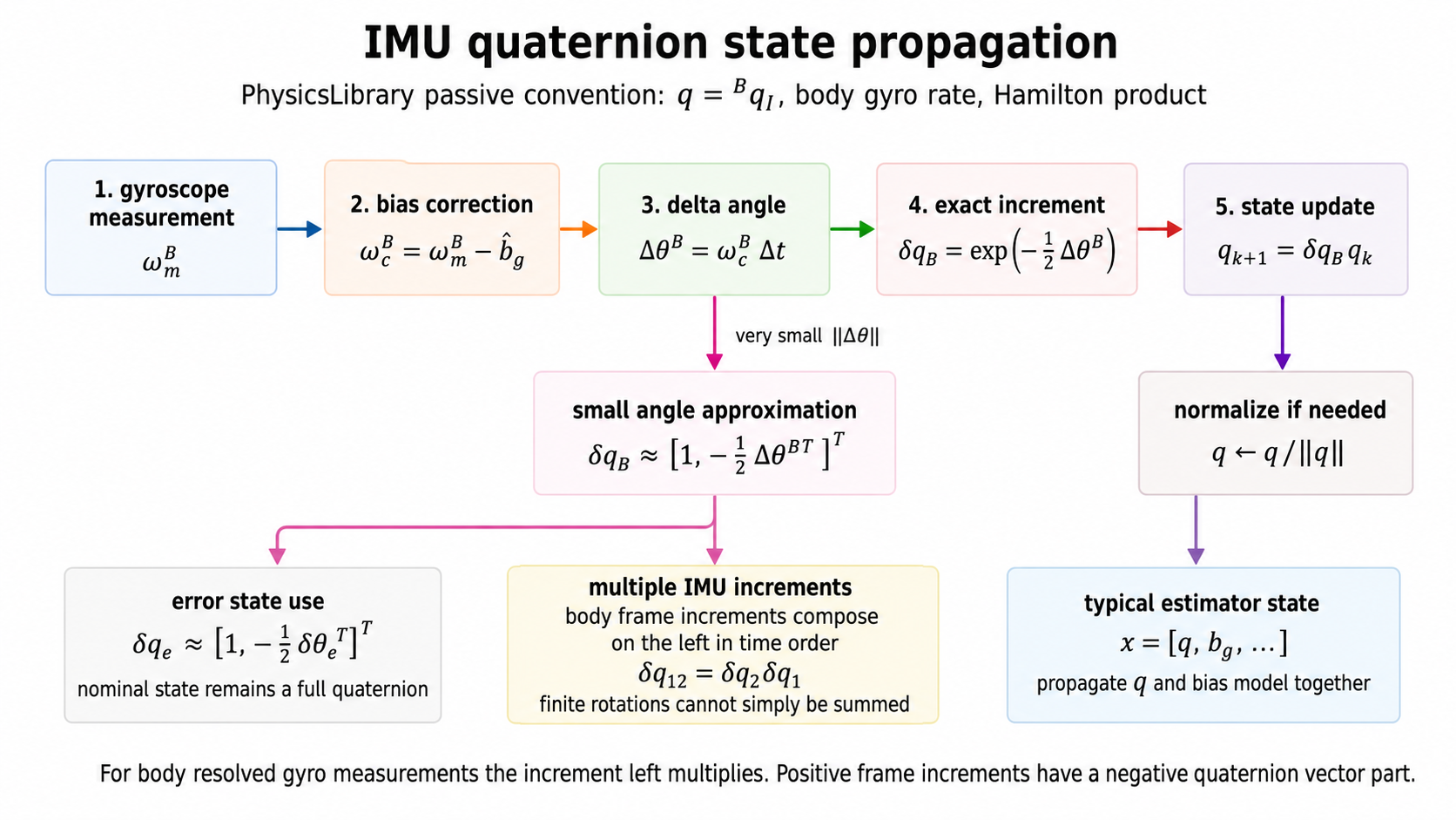
The following diagram summarizes the passive IMU attitude state propagation chain.

\includegraphics[width=0.97\textwidth]{Q13_imu_attitude_state_propagation.png}

Figure. A body mounted IMU supplies angular motion and specific force. Gyroscope bias is removed, a passive incremental quaternion is formed, and the increment left multiplies the inertial to body attitude quaternion. The updated or appropriately time centered attitude is then used to transform body specific force into the navigation or inertial frame. A multiplicative estimator may carry a three component local error state while the nominal orientation remains a full unit quaternion.

Small angle increment

For sufficiently small $\Delta\theta$,

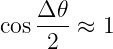
$\displaystyle \cos\frac{\Delta\theta}{2} \approx 1 $

and

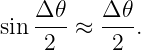
$\displaystyle \sin\frac{\Delta\theta}{2} \approx \frac{\Delta\theta}{2}. $

Therefore

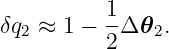
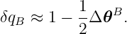
$\displaystyle \delta q_B \approx 1 - \frac12 \Delta\boldsymbol\theta^B.$ (19)

The corresponding first order update is

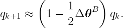
$\displaystyle q_{k+1} \approx \left( 1 - \frac12 \Delta\boldsymbol\theta^B \right) q_k.$ (20)

This is useful for analysis and for sufficiently small sample increments, but the exact trigonometric increment is inexpensive and generally preferable when the delta angle is already available.

Forward Euler integration

Starting from

$\displaystyle \dot q = -\frac12 \omega^B q, $

a forward Euler step is

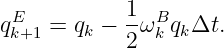
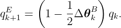
$\displaystyle q_{k+1}^{E} = q_k - \frac12 \omega_k^B q_k \Delta t.$ (21)

If

$\displaystyle \Delta\boldsymbol\theta_k^B = \omega_k^B\Delta t, $

then

$\displaystyle q_{k+1}^{E} = \left( 1 - \frac12 \Delta\boldsymbol\theta_k^B \right) q_k.$ (22)

Thus forward Euler is equivalent to using the first order incremental quaternion without normalization.

Why forward Euler leaves unit norm

The exact quaternion derivative is tangent to the unit quaternion three sphere.

A forward Euler method advances along the tangent line:

$\displaystyle q_{k+1}^{E} = q_k+\dot q_k\Delta t. $

For unit $q_k$,

$\displaystyle q_k^T\dot q_k=0. $

Therefore

\begin{equation*} \begin{aligned} \left\lVert q_{k+1}^{E} \right\rVert^2 &= \lef... ...1 + \left\lVert \dot q_k \right\rVert^2 \Delta t^2. \end{aligned}\end{equation*}

Hence

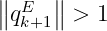
$\displaystyle \left\lVert q_{k+1}^{E} \right\rVert > 1$ (23)

for a nonzero rate and nonzero step.

The norm defect is second order for one step but accumulates during repeated propagation.

Normalization

A common numerical correction is

$\displaystyle q \leftarrow \frac{q}{\lVert q\rVert}.$ (24)

Normalization restores the unit quaternion constraint and is generally appropriate after an approximate propagation method or after finite precision arithmetic.

However, normalization does not make an approximate integration method identical to the exact exponential update. It restores the manifold constraint but does not reconstruct higher order phase terms omitted by the integrator.

For an exact unit incremental quaternion multiplying an exactly unit state, the product is analytically unit:

$\displaystyle \lVert \delta q_Bq_k \rVert = 1.$ (25)

Practical software may still normalize occasionally or every sample to control floating point drift.

A numerically stable small angle evaluation

Directly evaluating

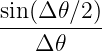
$\displaystyle \frac{\sin(\Delta\theta/2)}{\Delta\theta} $

can lose numerical quality when $\Delta\theta$ is extremely small.

Its Taylor expansion is

$\displaystyle \frac{ \sin(\Delta\theta/2) }{ \Delta\theta } = \frac12 - \frac{ \Delta\theta^2 }{48} + \frac{ \Delta\theta^4 }{3840} + O(\Delta\theta^6).$ (26)

Similarly,

$\displaystyle \cos\frac{\Delta\theta}{2} = 1 - \frac{ \Delta\theta^2 }{8} + \frac{ \Delta\theta^4 }{384} + O(\Delta\theta^6).$ (27)

A robust implementation may switch to such series below a small threshold.

Runge Kutta propagation

A higher order integrator can be applied directly to

$\displaystyle \dot q=f(q,t) = -\frac12 \omega^B(t)q.$ (28)

For classical fourth order Runge Kutta,

$\displaystyle k_1 = f(q_k,t_k),$ (29)
$\displaystyle k_2 = f \left( q_k+\frac{\Delta t}{2}k_1, t_k+\frac{\Delta t}{2} \right),$ (30)
$\displaystyle k_3 = f \left( q_k+\frac{\Delta t}{2}k_2, t_k+\frac{\Delta t}{2} \right),$ (31)
$\displaystyle k_4 = f \left( q_k+\Delta t\,k_3, t_k+\Delta t \right),$ (32)

and

$\displaystyle q_{k+1} = q_k + \frac{\Delta t}{6} \left( k_1+2k_2+2k_3+k_4 \right).$ (33)

The resulting quaternion should be normalized.

Runge Kutta methods are useful when an angular rate model can be evaluated inside the interval. If an IMU supplies only one integrated delta angle per sample, the exact finite incremental quaternion is often a more natural attitude update.

Exact update for a constant positive $z$ rate

Suppose

$\displaystyle q_0=1 $

and the body rotates at constant positive rate

$\displaystyle \omega^B = \Omega\mathbf k. $

Over one interval,

$\displaystyle \Delta\boldsymbol\theta^B = \Omega\Delta t\,\mathbf k. $

The increment is

$\displaystyle \delta q_B = \cos\frac{\Omega\Delta t}{2} - \mathbf k \sin\frac{\Omega\Delta t}{2}.$ (34)

After $N$ equal intervals,

$\displaystyle q_N = \cos\frac{\Omega N\Delta t}{2} - \mathbf k \sin\frac{\Omega N\Delta t}{2}.$ (35)

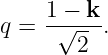
At a total positive frame rotation of $90^\circ$,

$\displaystyle q = \frac{ 1-\mathbf k }{ \sqrt2 }.$ (36)

This is the same passive convention diagnostic used throughout the preceding PhysicsLibrary quaternion series.

Using IMU supplied delta angles

Many inertial sensors report integrated angular increments directly:

$\displaystyle \Delta\boldsymbol\theta_m^B.$ (37)

Such an output may already incorporate internal high rate sampling and manufacturer specific coning processing.

If the bias estimate is expressed as an angular rate and is approximately constant over the sample, a simple correction is

$\displaystyle \Delta\widehat{\boldsymbol\theta}^B = \Delta\boldsymbol\theta_m^B - \widehat{\mathbf b}_g \Delta t.$ (38)

The corrected delta angle is then converted directly to the passive incremental quaternion.

The device documentation must be checked to determine whether its reported increment is raw, internally compensated, expressed in a beginning sample frame, expressed in an ending sample frame, or uses another convention.

Gyroscope bias accumulation

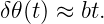
If an uncompensated constant gyro bias has magnitude $b$, then for a simple single axis case the attitude error grows approximately as

$\displaystyle \delta\theta(t) \approx bt.$ (39)

For example, a bias of

$\displaystyle 0.1^\circ/\mathrm{s} $

accumulates approximately

$\displaystyle 60^\circ $

of angle error in ten minutes.

This simple calculation explains why accurate bias initialization, online bias estimation, temperature modeling, and external aiding are important in inertial systems.

Two successive body increments and coning

Consider two small chronological body frame increments

$\displaystyle \Delta\boldsymbol\theta_1 $

followed by

$\displaystyle \Delta\boldsymbol\theta_2. $

The passive incremental quaternions are
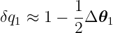
$\displaystyle \delta q_1 \approx 1-\frac12\Delta\boldsymbol\theta_1 $

and

$\displaystyle \delta q_2 \approx 1-\frac12\Delta\boldsymbol\theta_2. $

Because body increments left multiply, the chronological combined update is

$\displaystyle q_2 = \delta q_2 \delta q_1 q_0.$ (40)

Expand the increment product through second order:
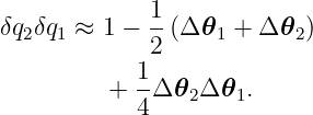
\begin{equation*} \begin{aligned} \delta q_2\delta q_1 \approx{}& 1 - \frac12 \l... ...Delta\boldsymbol\theta_2 \Delta\boldsymbol\theta_1. \end{aligned}\end{equation*}

The vector part of the last product is

$\displaystyle \frac14 \left( \Delta\boldsymbol\theta_2 \times \Delta\boldsymbol... ...c14 \left( \Delta\boldsymbol\theta_1 \times \Delta\boldsymbol\theta_2 \right). $

Matching the passive first order form
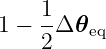
$\displaystyle 1-\frac12 \Delta\boldsymbol\theta_{\mathrm{eq}} $

gives the leading equivalent physical rotation vector

$\displaystyle \Delta\boldsymbol\theta_{\mathrm{eq}} \approx \Delta\boldsymbol\t... ...l\theta_2 + \frac12 \Delta\boldsymbol\theta_1 \times \Delta\boldsymbol\theta_2.$ (41)

The cross product term is the leading coning contribution.

Why coning matters

If the body rotates alternately about different axes during a sample interval, the vector sum of the measured increments is not generally the exact net rotation.

The missing information appears first through cross products of successive angular increments.

High accuracy strapdown inertial algorithms therefore use multiple subsamples or compensated delta angles to account for noncommutativity.

A simple one sample exponential update is exact for a constant rotation vector over the interval. It is not automatically exact for arbitrary high frequency motion occurring within that interval.

If an IMU already reports a coning compensated delta angle, applying an additional naive coning correction may double count the effect.

Attitude sign continuity

The unit quaternions

$\displaystyle q $

and

$\displaystyle -q $

represent the same physical orientation.

A numerical quaternion time history may therefore contain equivalent samples with alternating overall signs.

For plotting, interpolation, finite differencing, or optimization, choose the representative nearest the previous sample.

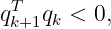
If

$\displaystyle q_{k+1}^Tq_k<0,$ (42)

replace

$\displaystyle q_{k+1} \leftarrow -q_{k+1}.$ (43)

This does not change the physical attitude.

Sign continuity is a representation choice. It is distinct from quaternion normalization and from selecting the principal error quaternion in a local attitude error calculation.

Specific force transformation

An accelerometer rigidly attached to the body reports specific force resolved in body coordinates:

$\displaystyle {}^{B}\mathbf f.$ (44)

The passive attitude quaternion maps inertial coordinates into body coordinates, so the inverse DCM maps body coordinates back into inertial coordinates:

$\displaystyle {}^{I}\mathbf f = {}^{I}C_B \,{}^{B}\mathbf f = ({}^{B}C_I)^T {}^{B}\mathbf f.$ (45)

Since

$\displaystyle {}^{B}C_I=C(q), $

we have

$\displaystyle {}^{I}\mathbf f = C(q)^T {}^{B}\mathbf f.$ (46)

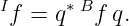
The equivalent quaternion sandwich is

$\displaystyle {}^{I}f = q^* \,{}^{B}f \,q.$ (47)

This inversion is important: the quaternion used for attitude propagation maps $I\rightarrow B$, while navigation mechanization often needs to rotate a measured body vector $B\rightarrow I$.

Velocity and position propagation

In a simple inertial frame model,

$\displaystyle {}^{I}\dot{\mathbf v} = {}^{I}\mathbf f + {}^{I}\mathbf g,$ (48)

and

$\displaystyle {}^{I}\dot{\mathbf r} = {}^{I}\mathbf v.$ (49)

In a rotating navigation frame, Earth rotation, transport rate, Coriolis terms, and the chosen gravity model must also be included.

A typical strapdown propagation cycle is therefore:

  1. read gyroscope and accelerometer information;
  2. correct the gyroscope data for estimated bias;
  3. form or accept a corrected body delta angle;
  4. update the passive attitude quaternion;
  5. obtain an attitude appropriate to the accelerometer integration time;
  6. transform specific force from body coordinates into the navigation or inertial frame;
  7. add gravity and required rotating frame terms;
  8. integrate velocity and position;
  9. propagate bias and other estimator states.

Why time centered attitude can matter

Using only the beginning or ending attitude to transform accelerometer data introduces an error when the body rotates appreciably during the sample.

For constant body rate, a midpoint quaternion can be formed as

$\displaystyle q_{k+1/2} = \delta q_{1/2} q_k,$ (50)

where

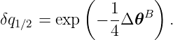
$\displaystyle \delta q_{1/2} = \exp \left( -\frac14 \Delta\boldsymbol\theta^B \right).$ (51)

The corresponding midpoint DCM can then be used for a simple time centered specific force transformation.

High accuracy inertial algorithms develop this idea further through sculling compensation and multiple sample integration.

Nominal quaternion and three component error state

A navigation filter can propagate the nominal attitude as a full unit quaternion while carrying only three attitude error states.

For example, using the passive small error convention from the preceding article,

$\displaystyle \delta q \approx \begin{bmatrix} 1\ -\frac12 \delta\boldsymbol\theta \end{bmatrix}.$ (52)

The nominal quaternion supplies a globally nonsingular orientation representation, while

$\displaystyle \delta\boldsymbol\theta $

is a local three component perturbation suitable for linear covariance propagation.

The chosen left or right error definition must remain consistent with the filter Jacobians and the side used for correction injection.

Direct small increment versus error state small angle

The same small angle expansion appears in two distinct roles.

In direct IMU propagation,
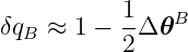
$\displaystyle \delta q_B \approx 1-\frac12 \Delta\boldsymbol\theta^B $

approximates the actual physical incremental rotation during one sample. Its accuracy depends on the size and variation of the sample motion.

In an error state filter,
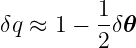
$\displaystyle \delta q \approx 1-\frac12 \delta\boldsymbol\theta $

represents a deliberately local estimation error around a nominal full attitude quaternion.

The nominal vehicle attitude itself may be very large even when the local error state is small.

These two uses should not be conflated.

Normalization versus sign continuity

Two common operations have different purposes.

Normalization,

$\displaystyle q \leftarrow \frac{q}{\lVert q\rVert}, $

restores the unit norm constraint.

Sign continuity,

$\displaystyle q_k\leftarrow-q_k $

when needed, chooses one of two equivalent quaternion representatives.

Neither operation substitutes for an accurate attitude integration method.

Example propagation step

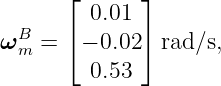
Suppose

$\displaystyle q_k=1, $

$\displaystyle \boldsymbol\omega_m^B = \begin{bmatrix} 0.01\ -0.02\ 0.53 \end{bmatrix}\mathrm{rad/s}, $

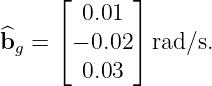
and

$\displaystyle \widehat{\mathbf b}_g = \begin{bmatrix} 0.01\ -0.02\ 0.03 \end{bmatrix}\mathrm{rad/s}. $

The corrected rate is

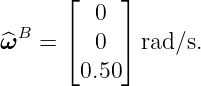
$\displaystyle \widehat{\boldsymbol\omega}^B = \begin{bmatrix} 0\ 0\ 0.50 \end{bmatrix}\mathrm{rad/s}.$ (53)

For

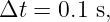
$\displaystyle \Delta t=0.1\ \mathrm{s}, $

the delta angle is

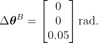
$\displaystyle \Delta\boldsymbol\theta^B = \begin{bmatrix} 0\ 0\ 0.05 \end{bmatrix}\mathrm{rad}.$ (54)

Therefore

$\displaystyle \delta q_B = \cos0.025 - \mathbf k\sin0.025.$ (55)

Numerically,

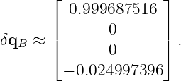
$\displaystyle \delta\mathbf q_B \approx \begin{bmatrix} 0.999687516\ 0\ 0\ -0.024997396 \end{bmatrix}.$ (56)

Since the initial attitude is the identity,

$\displaystyle q_{k+1} = \delta q_Bq_k = \delta q_B.$ (57)

Forward Euler comparison for the same step

The forward Euler result is

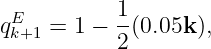
$\displaystyle q_{k+1}^{E} = 1 - \frac12 (0.05\mathbf k), $

so

$\displaystyle q_{k+1}^{E} = 1 - 0.025\mathbf k.$ (58)

Its norm is

$\displaystyle \left\lVert q_{k+1}^{E} \right\rVert = \sqrt{1.000625} \approx 1.000312451.$ (59)

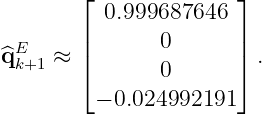
After normalization,

$\displaystyle \widehat{\mathbf q}_{k+1}^{E} \approx \begin{bmatrix} 0.999687646\ 0\ 0\ -0.024992191 \end{bmatrix}.$ (60)

This is close to, but not identical with, the exact exponential result.

Implementation pseudocode

A minimal constant rate passive update can be expressed conceptually as:

omega_B = gyro_B - bias_hat_B
dtheta_B = omega_B * dt
a = norm(dtheta_B)

if a is very small:
s = 0.5 - a*a/48
c = 1.0 - a*a/8
else:
s = sin(a/2) / a
c = cos(a/2)

dq = [c, -s*dtheta_B]
q_new = dq * q_old
q_new = q_new / norm(q_new)

if dot(q_new, q_old) < 0:
q_new = -q_new

The product in the line

$\displaystyle \texttt{q\_new = dq * q\_old} $

is the Hamilton product with scalar first semantic components.

Software whose array order is scalar last may use different memory indices without changing the physical equations.

Common pitfalls

  1. Using the old inverse attitude convention.

    The present PhysicsLibrary state is

    $\displaystyle q={}^Bq_I, $

    not ${}^Iq_B$.

  2. Using a positive vector part for a positive body frame increment.

    The passive increment is

    $\displaystyle \delta q_B = \cos\frac{\Delta\theta}{2} - \widehat{\mathbf u} \sin\frac{\Delta\theta}{2}. $
  3. Right multiplying body resolved increments.

    For the passive inertial to body state,

    $\displaystyle q_{k+1} = \delta q_Bq_k. $
  4. Assuming normalization makes Euler integration exact.

    Normalization repairs norm, not truncation error.

  5. Ignoring gyro bias.

    Even a small constant rate bias integrates into a large attitude error over time.

  6. Applying a simple vector sum to substantial multi axis motion.

    Successive rotations do not commute. Coning terms matter.

  7. Applying coning correction twice.

    Determine whether the sensor supplied delta angle already contains internal compensation.

  8. Using the inertial to body quaternion in the wrong direction for accelerometer data.

    Body specific force is transformed to inertial coordinates with $q^*$ on the left and $q$ on the right, or with $C(q)^T$.

  9. Interpreting quaternion sign flips as attitude jumps.

    $q$ and $-q$ represent the same orientation.

  10. Treating the three component filter attitude error as the nominal attitude itself.

    The error vector is local; the nominal quaternion carries the global orientation.

Verification battery

A numerical implementation should be checked against:

  1. zero angular rate;
  2. constant positive rotations about $+x$, $+y$, and $+z$;
  3. exact exponential propagation from the identity;
  4. equality of $C(q_{k+1})$ with the equivalent DCM increment;
  5. preservation of unit norm for exact increments;
  6. expected norm drift for unnormalized forward Euler;
  7. gyro bias accumulation;
  8. body increment multiplication on the left;
  9. sign continuity with $q$ versus $-q$;
  10. two noncommuting increments and the leading coning term;
  11. specific force transformation with the inverse attitude map;
  12. consistency with the passive error state sign from Q12.

Relationship to adjacent PhysicsLibrary entries

The preceding article, Relative Attitude and Error Quaternions, establishes multiplicative left and right errors and the passive local relation
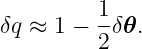
$\displaystyle \delta q \approx 1-\frac12\delta\boldsymbol\theta. $

The present article combines that convention with the quaternion kinematics from quaternion kinematics and angular velocity to form sampled IMU attitude propagation.

A separate companion entry, Numerical Quaternion Propagation and IMU Attitude State Integration: Examples, Exercises, and Solutions, provides the Q13E self study problem bank.

Sources and convention notes

Quaternion propagation equations cannot be imported safely without identifying the represented frame map, the resolution of angular velocity, and the quaternion multiplication convention.

Sommer and coauthors provide a modern discussion of convention management. Solà provides a detailed treatment of quaternion kinematics and IMU error state filtering. Titterton and Weston provide a broad engineering treatment of strapdown inertial navigation. Savage develops the classical strapdown attitude integration framework, including coning compensation.

The equations in this entry are translated into the PhysicsLibrary passive inertial to body convention.

Bibliography

1
H. Sommer, I. Gilitschenski, M. Bloesch, S. Weiss, R. Siegwart, and J. Nieto, “Why and How to Avoid the Flipped Quaternion Multiplication,” Aerospace, vol. 5, no. 3, article 72, 2018. Published under CC BY 4.0. Publisher article https://www.mdpi.com/2226-4310/5/3/72
2
J. Solà, “Quaternion Kinematics for the Error State Kalman Filter,” arXiv:1711.02508, 2017. arXiv preprint https://arxiv.org/abs/1711.02508
3
D. H. Titterton and J. L. Weston, Strapdown Inertial Navigation Technology, 2nd ed., The Institution of Engineering and Technology, 2004/2005. Engineering reference. IET book page https://shop.theiet.org/strapdn-inertial-navig-t-2ed
4
P. G. Savage, “Strapdown Inertial Navigation Integration Algorithm Design Part 1: Attitude Algorithms,” Journal of Guidance, Control, and Dynamics, vol. 21, no. 1, pp. 19–28, 1998. DOI record https://doi.org/10.2514/2.4228

License

Unless otherwise noted, this PhysicsLibrary entry is intended for release under the Creative Commons Attribution ShareAlike 4.0 International license.


"numerical quaternion propagation and IMU attitude state integration" is owned by bloftin.
(view preamble)
View style:
See Also: quaternion series overview and article guide, Notation Quaternions for Physics and Engineering: Orientation, quaternion definition and basic algebra, example of quaternion definition and basic algebra

Keywords:  quaternion, numerical propagation, IMU, gyroscope, attitude state, delta angle, small angle approximation, coning correction, inertial navigation, strapdown navigation

Attachments:
example of numerical quaternion propagation and IMU attitude state integration (Example) by bloftin

Cross-references: quaternion multiplication, quaternion kinematics and angular velocity, kinematics, relation, commute, operations, injection, covariance, position, error quaternion, representation, algorithms, cross product, temperature, magnitude, manifold, norm, force, diagram, composition, identity, scalar, vector, velocity, reference frame, Euler Angle, quaternions, system, motion
There are 3 references to this object.

This is version 4 of numerical quaternion propagation and IMU attitude state integration, born on 2026-08-24, modified 2026-08-28.
Object id is 1109, canonical name is NumericalQuaternionPropagationAndIMUAttitudeStateIntegration.
Accessed 91 times total.

Classification:
Physics Classification45.40.-f (Dynamics and kinematics of rigid bodies)
 02.40.Yy (Geometric mechanics )
 06.30.Gv (Velocity, acceleration, and rotation)
Pending Errata and Addenda
None.
Discussion
Style: Expand: Order:

No messages.

Interact
rate | post | correct | update request | add example | add (any)