FS20: Equivalence of Real and Complex Fourier Forms
The real Fourier series and the complex Fourier series are not two different theories of periodic
functions. They describe the same harmonic components using different coordinates. In FS04–FS06
we extracted coefficients of cosine and sine functions. FS18 rewrote those functions as
oppositely rotating complex exponentials, and FS19 derived the complex coefficients
by orthogonal projection. Now we will join those two developments into a reversible
calculation.
A key conceptual question is this: if a real signal has one cosine-and-sine harmonic at frequency n,
why does its complex spectrum have two coefficients, one at +n and one at −n? The answer is not
additional physical energy or a new frequency. It is a different bookkeeping system for the very
same real oscillation.
The central results we will earn for n ≥ 1 are
and
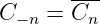
We will also show that C0 = a0∕2 and, for real-valued f, that C−n = Cn.
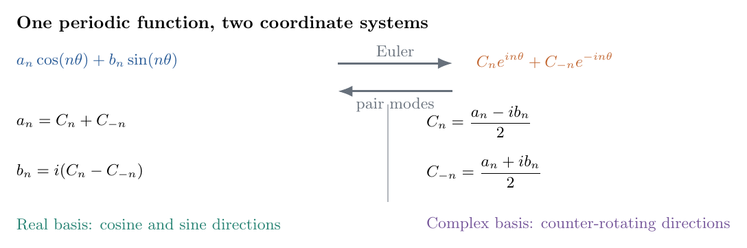
Figure 1. The real and complex descriptions are two invertible coordinate systems for one
harmonic. Neither introduces a new physical oscillation.
1 Begin with the two formulas on the same interval
Let f be a real-valued, 2L-periodic function. Write
We use 𝜃 only as an abbreviation; the period in x remains 2L. The real Fourier form
is
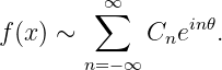
The complex Fourier form is
In the first sum, the index starts at 1, and there are two real coefficients for each positive
harmonic. In the second sum, the index spans all integers and there is one complex coefficient for
each signed harmonic. The complex sum also contains n = 0.
When making algebraic transformations, begin with finite sums. This avoids silently exchanging
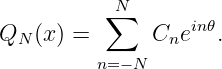
infinite sums or limits. Set
and
Our first task is to choose Cn so that QN(x) = RN(x) identically, for every x, without taking N to
infinity.
2 One cosine requires a positive and a negative frequency
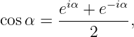
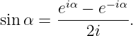
Euler’s formula reads
Changing the sign of α gives
Add these equations. The imaginary terms cancel:
Subtract instead. The real parts cancel:
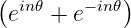
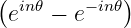
Therefore
and
These are identities, not approximations.
An important geometric point follows. The phasor ein𝜃 rotates counterclockwise as 𝜃
increases for positive n, while e−in𝜃 rotates in the opposite direction. Their sum has no
imaginary component and produces a cosine. Their suitably scaled difference produces a
sine.
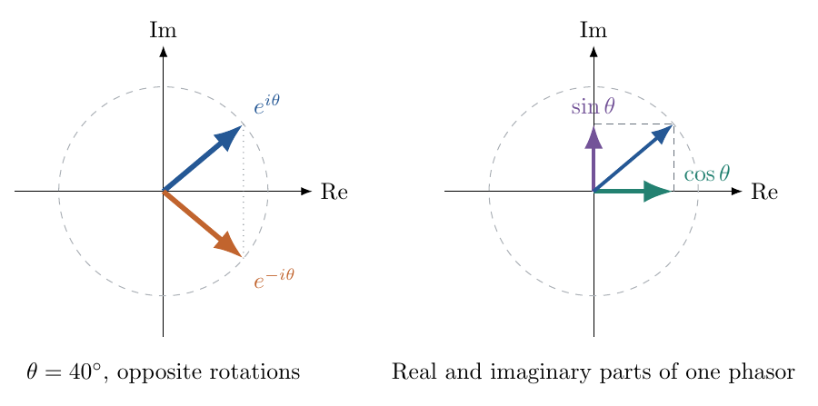
Figure 2. Euler’s formula relates complex rotation to real cosine and sine components. A real
sinusoid can be assembled from a conjugate pair of counter-rotating complex modes.
3 Derive the conversion from real coefficients to complex coefficients
Take just one real harmonic, not the whole series:
Replace cosine and sine using Equations (12) and (13):
The only algebraic subtlety is that
because i(−i) = 1. Therefore the sine part can be rewritten as
Now collect the multiplier of ein𝜃 and the multiplier of e−in𝜃:
| hn(x) | = 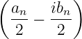 ein𝜃 | |
|
| + 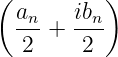 e−in𝜃. | (18) |
Compare this equation with
The coefficients must be
and
What happens to the constant term?
At zero frequency, ei0𝜃 = 1. There is only one zero-frequency mode, not a positive-negative pair.
The constant term in Equation (6) is already a0∕2. Thus
Do not apply Equation (20) at n = 0 while also inventing a separate C−0. That would count the
DC component twice.
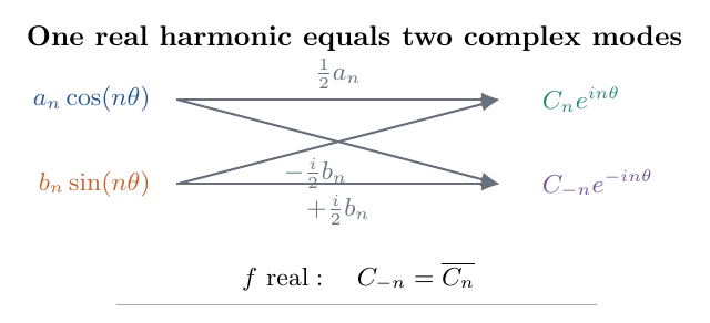
Figure 3. The real cosine coefficient contributes equally to +n and −n, while the real sine
coefficient contributes oppositely signed imaginary parts.
4 Derive the reverse conversion from complex to real
Now suppose the complex coefficients Cn and C−n are known. Start with the two equations just
obtained:
Add them:
so
Subtract the second equation from the first:
Divide by −2i, or multiply by i∕2:
Finally,
The two forms are therefore related by a reversible linear change of coordinates. We did not
approximate anything in either direction.
Why real signals have conjugate pairs
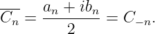
For a real-valued function, the Fourier coefficients an and bn are real numbers. Conjugating
Equation (20) gives
Consequently,
and
The minus sign in the formula for bn follows from our e+in𝜃 synthesis convention. Other Fourier
sign conventions can reverse it, so the safe approach is to derive the conversion once from Euler’s
formula.
We can verify the real-valued nature of a conjugate pair directly:
| Cnein𝜃 + C
−ne−in𝜃 | = C
nein𝜃 + C
nein𝜃 | |
|
| = 2 Re  . | (33) |
Thus a conjugate pair is exactly the real harmonic an cos(n𝜃) + bn sin(n𝜃).
5 Worked example 1: reconstruct a finite signal both ways
Reuse the FS19 waveform
From the real form we read
with every other nonzero-index coefficient equal to zero. Use our conversion formulas one harmonic
at a time.
At zero frequency,
At the first harmonic, b1 = 0, giving
At the second harmonic, a2 = 0 and b2 = −2, giving
Thus the complex form is the finite expression
Group the pair at n = ±1:
Group the pair at n = ±2:
We recover Equation (34) exactly.
As an independent check, use the reverse formulas. For n = 2,
and
Notice how the sine coefficient is stored as imaginary components with opposite signs in the
complex spectrum.
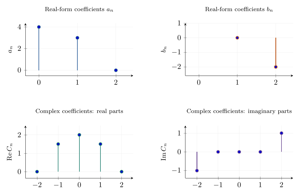
Figure 4. The same finite signal written in real and complex coefficient form. The zero-frequency
real coefficient is a0 = 4 whereas C0 = 2; the other harmonics are divided between paired positive
and negative frequencies.
6 Amplitude and phase: interpreting a complex coefficient
We often express one real harmonic as
Expand the cosine of a difference:
| hn(x) | = An cos φn cos(n𝜃) | |
|
| + An sin φn sin(n𝜃). | (45) |
Compare with an cos(n𝜃) + bn sin(n𝜃) to identify
Therefore
The phase φn is chosen with the correct quadrant, for example using the two-argument arctangent
atan2(bn,an).
Substitute Equation (46) into the complex conversion:
Hence
The complex spectrum has two conjugate coefficients of magnitude An∕2, but the real sinusoid has
amplitude An. It would be wrong to read |Cn| alone as the real amplitude without accounting for
the negative-frequency partner.
A quick phase example
Take
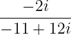
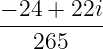
The real coefficients are a1 =  and b1 = 1. The complex coefficients are
Each has magnitude 1, while the recovered real sinusoid has amplitude 2. The negative argument
of C1 is consistent with our cos(x − φ) phase convention.
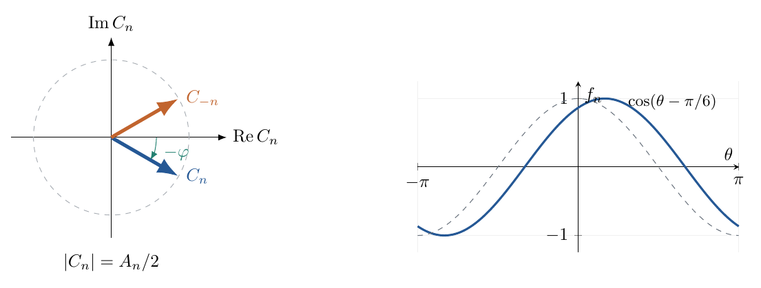
Figure 5. A positive-frequency coefficient and its conjugate form symmetric phasors. The
coefficient phase records the shift of the real sinusoid; two complex magnitudes An∕2 combine to
recover amplitude An.
7 Worked example 2: the odd square wave
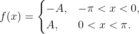
Recall from FS07 the odd square wave of amplitude A on [−π,π]:
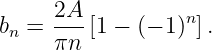
It is odd, so a0 = an = 0. Its sine coefficients are
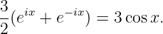
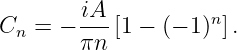
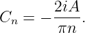
For positive n, the complex coefficient is therefore
For odd positive n this reduces to
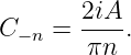
Its negative-frequency partner is
Both even-harmonic coefficients are zero; the conjugate pair at each odd harmonic recreates the
sine term. Notice that |Cn| = 2A∕(πn) whereas the real sine amplitude is bn = 4A∕(πn).
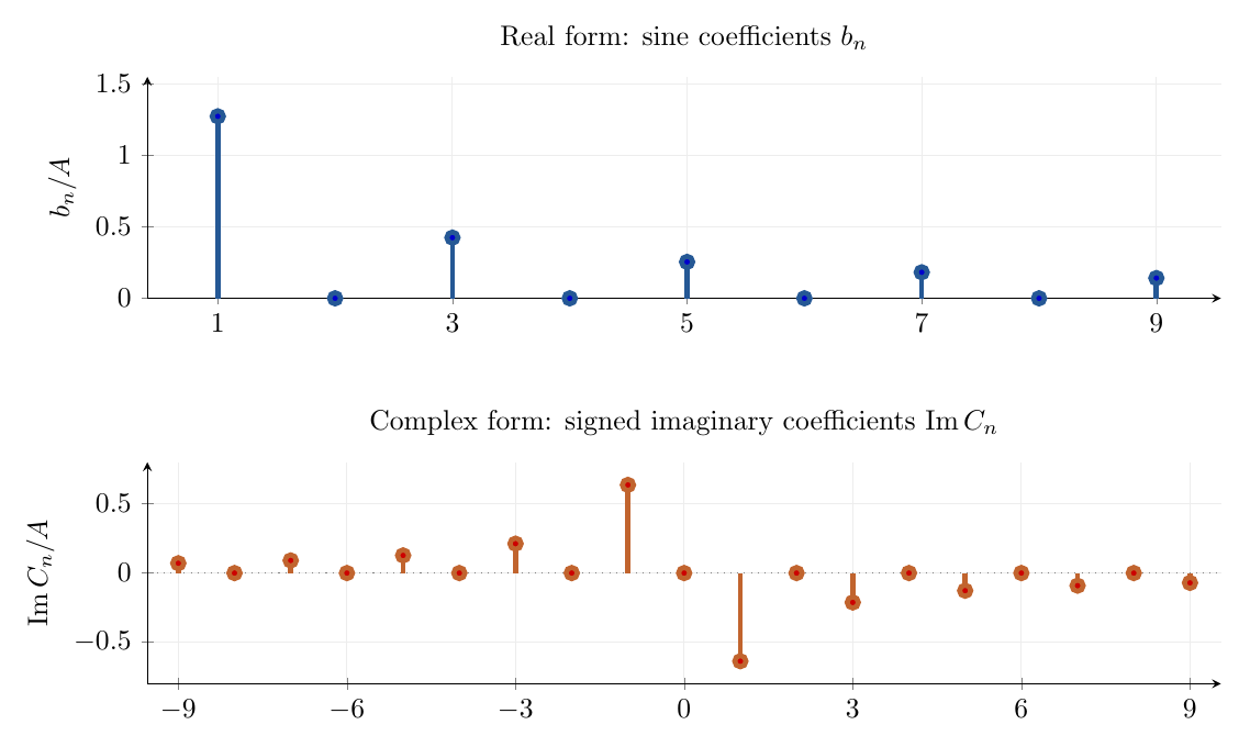
Figure 6. The real odd square wave has positive coefficients on odd sine harmonics. Its complex
spectrum stores them as an antisymmetric imaginary pair at positive and negative indices. The
vertical scales reflect the factor of two.
8 Worked example 3: an even rectangular pulse
Define a periodic centered pulse by
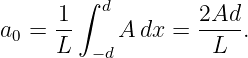
Because the pulse is even, all bn = 0. Its constant term is
For n ≥ 1 the cosine coefficient is
| an | =  ∫
0d cos  dx | |
|
| =  sin  . | (59) |
Thus the complex coefficients are
and
These coefficients are real and even in their index. This is the spectral signature of an even, real
waveform about the chosen origin. The sign of a coefficient can still be negative, so a plot of
coefficient magnitude alone loses information.
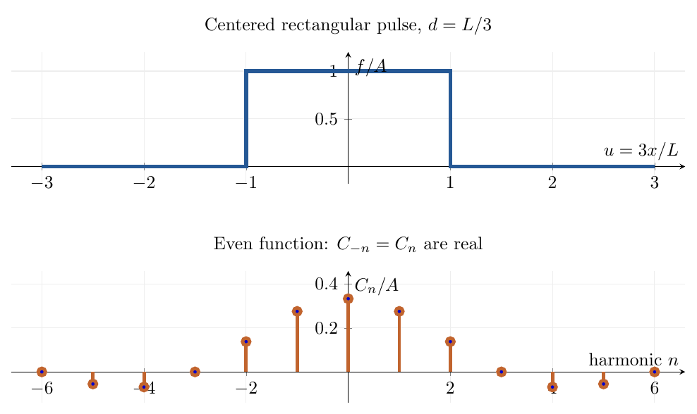
Figure 7. A centered even pulse and its real, even two-sided complex coefficient sequence. The
horizontal waveform coordinate u = 3x∕L is used for the illustrated choice d = L∕3.
9 Time shifts change phase, not coefficient magnitude
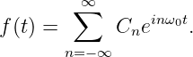
For a periodic time signal, replace 𝜃 by ω0t, where ω0 = 2π∕T. Suppose
Shift the entire waveform to the right by t0:
| g(t) | = f(t − t0) | |
|
| = ∑
nCneinω0(t−t0) | |
|
| = ∑
n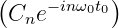 einω0t. | (63) |
Therefore
Since |e−inω0t0| = 1, the magnitude stays unchanged:
A delay changes the phases by −nω0t0; harmonics at higher n rotate farther.
To see the same transformation in real coefficients, set α = nω0t0 and expand a single shifted
harmonic. One finds
These formulas are a rotation in the (an,bn) coefficient plane. In the complex plane, the same
rotation is expressed more economically by multiplication by one exponential.
A quick check
Start with f(t) = cos(ω0t) and delay by T∕4. Then α = π∕2, and the shifted waveform is sin(ω0t).
The real formulas yield a1(g) = 0 and b
1(g) = 1. The complex formula yields C
1(g) = −i∕2,
C−1(g) = i∕2. Both descriptions agree.
10 Finite energy bookkeeping also agrees
FS12 established that orthogonal projection splits the squared norm among retained directions.
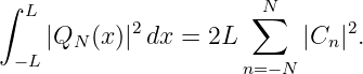
For a real Fourier partial sum on [−L,L], orthogonality gives
Using the complex basis, whose squared norm is 2L, we obtain
But the finite sums are the same function. The right sides must agree. Indeed, for each positive
n,
| |Cn|2 + |C
−n|2 | =  +  | |
|
| =  . | (70) |
Multiplying by 2L gives precisely L(an2 + b
n2). The DC contribution is 2L|C
0|2 = La
02∕2.
This identity is finite, so it does not yet require a theorem about the convergence of the infinite
Fourier series. FS13 develops the infinite-series energy statement, Parseval’s theorem, under the
appropriate completeness assumptions.
11 What if the function itself is complex-valued?
Our algebraic identities converting an,bn and C±n do not require f to be real, provided the
real-form coefficients are allowed to be complex. However, the symmetry
does require the signal to be real-valued (in the usual almost-everywhere sense). For
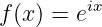
example,
has C1 = 1 and C−1 = 0. This is perfectly valid for a complex signal; no conjugate partner is
required.
Complex signals are useful mathematical objects, and in electronics the in-phase/quadrature signal
is commonly represented as a complex envelope. The physical meaning of this complex notation
depends on the system and should not be confused with the automatically real quantity
Re{ei𝜃}.
12 Physics example: periodic forcing of a damped oscillator
Consider the linear mass-spring-damper equation
Suppose the forcing is a real periodic signal of fundamental angular frequency ω0. Write the
complex expansions
For each exponential, differentiation multiplies by inω0; differentiating twice multiplies by
−(nω0)2. Consequently the equation for each harmonic becomes
For a stable forced response,
A numerical two-harmonic forcing
Let M = 1 kg, b = 2 N s∕m, k = 25 N∕m, and ω0 = 3 rad∕s. Apply
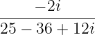
The nonzero force coefficients are
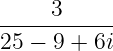
At n = 1, the response is
At n = 2,
The negative-frequency responses are their conjugates because the forcing and the system
coefficients are real. Convert the two positive-frequency coefficients back to the real
basis:
Therefore the real steady-state displacement is
| y(t) | =  cos(3t) +  sin(3t) | |
|
| − cos(6t) −  sin(6t), | (83) |
with displacement measured in meters. Direct substitution into Equation (73) reproduces the
original force.
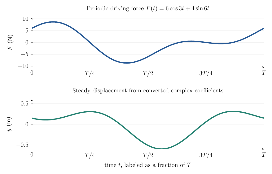
Figure 8. A two-harmonic periodic force and the corresponding steady displacement. Complex
coefficients make each harmonic response algebraic; conjugate pairing converts the result into the
real displacement observed in the laboratory.
13 Choosing which representation to use
The real form is often the more intuitive choice when drawing a waveform, separating even and
odd contributions, specifying a directly measured cosine or sine amplitude, or teaching elementary
harmonic synthesis. The complex form is usually more compact when differentiating harmonics,
handling shifts, keeping phase and amplitude together, or solving linear differential equations mode
by mode.
Neither form is intrinsically more accurate. Their finite partial sums are identical functions when
the coefficients are converted correctly. Any difference in an actual computation comes from
truncation, rounding, or using different conventions, not from a mathematical difference between
real and complex Fourier series.
Common convention traps
- Mixing C0 and a0: the constant term is C0 = a0∕2, not a0.
- Ignoring negative frequencies: for a real sinusoid, two complex exponentials reconstruct
one real harmonic.
- Forgetting the imaginary sign: with synthesis e+in𝜃, b
n = −2 Im Cn for positive n.
- Reading |Cn| as the real amplitude: for n ≥ 1, the real amplitude is 2|Cn|.
- Treating ein𝜃 as automatically real: a single complex exponential is generally complex;
reality requires conjugate pairing.
- Confusing series with transforms: a periodic signal has discrete harmonic indices. FS26
develops the different continuous-frequency Fourier transform.
14 Self-checks
- If f(x) = 5 + 4 cos 3x, find C0,C3,C−3 and all other nonzero coefficients. Answer:
C0 = 5, C±3 = 2.
- If C2 = 1 − 2i and f is real, what is C−2 and what real harmonic do they represent?
Answer: C−2 = 1 + 2i and 2 cos 2x + 4 sin 2x.
- What is the amplitude of a real harmonic whose positive-frequency coefficient has
modulus 0.4? Answer: 0.8.
- Can C−1 = 0 and C1 = 1 describe a real-valued waveform? Answer: not by themselves;
they give eix, a complex waveform.
- Why does cos x delayed by one quarter-period become sin x? Answer: the
positive-frequency coefficient rotates by e−iπ∕2 = −i; the real coefficient vector rotates
from (a1,b1) = (1, 0) to (0, 1).
15 What FS20 has established
From FS02’s projection idea to FS19’s complex coefficient formula, we have arrived at a
complete dictionary between real and complex representations. Euler’s formula pairs two
counter-rotating exponentials into one real harmonic. Their complex coefficients store both the
amplitude and phase, and their conjugate symmetry guarantees a real result. The finite
projection energy is identical in the two descriptions, and linear physical systems can
be solved harmonic by harmonic in complex form before returning to measurable real
variables.
This prepares two important directions: FS21 develops Fourier modes as eigenfunctions in
separation-of-variables problems, and FS26 explains how discrete harmonics become a
continuous-frequency integral for nonperiodic signals.
References
[1] E. Kreyszig, Advanced Engineering Mathematics, 10th ed., Wiley, 2011.
[2] R. N. Bracewell, The Fourier Transform and Its Applications, 3rd ed., McGraw-Hill,
2000.
[3] A. V. Oppenheim and A. S. Willsky, Signals and Systems, 2nd ed., Prentice Hall,
1997.
[4] G. B. Arfken, H. J. Weber, and F. E. Harris, Mathematical Methods for Physicists,
7th ed., Academic Press, 2012.




























































 =


 =