Electromagnetic Waves: Magnetic Fields Produced by Currents

Electromagnetic Waves, Antennas, and RF: Magnetic Fields Produced by Currents

EM10 treated the magnetic field B as an applied field and asked what force it exerts on moving charges and currents. EM11 reverses that viewpoint and asks a source problem:

|------------------------------------------------------| -How--does-an-electric-current produce-a-magnetic-field?--

(1)

For steady currents, the central tool is the Biot–Savart law. It plays a role for magnetostatics analogous to Coulomb’s law for electrostatics: a distributed source is broken into small source elements, the field produced by each element is computed, and the vector contributions are added by superposition [1, 2, 3, 5].

This article develops that construction carefully because the same source-point/observation-point geometry will reappear later in antenna theory. The important limitation is that the Biot–Savart law developed here is a magnetostatic law for steady currents. Time-varying antenna currents require the full time-dependent electromagnetic theory developed later in this series.

1 Current as a source of magnetic field

A stationary charge produces an electrostatic field. When charge moves in an organized current, magnetic fields are also produced.

The source strength is represented by current I. For a thin wire, an infinitesimal current element is written

′ I dℓ.

(2)

The prime reminds us that dℓ′ belongs to the source location. This distinction will matter whenever source and observation coordinates appear in the same equation.

The constant that sets the magnetic-field scale in vacuum is the vacuum permeability,

|-----------------------------| μ0 ≈ 1.25663706 × 10−6 H/m. | -------------------------------

(3)

Equivalent SI units may also be written as N/A².

2 Source point and observation point

Let the source current element be located at

r′,

(4)

and let the magnetic field be evaluated at the observation point

r.

(5)

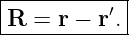
Define the separation vector

|------------| |R = r − r′. | -------------

(6)

Its magnitude is

R = |R |,

(7)

and its unit vector is

R ˆR = --. R

(8)

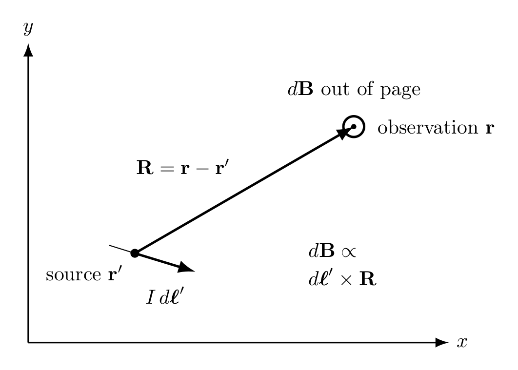
Figure. Biot–Savart geometry. A source current element I dℓ′ at r′ contributes a magnetic field at observation point r. The separation vector is R = r − r′.

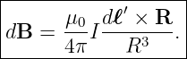
3 The Biot–Savart law

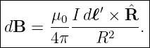
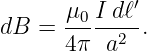
For a steady current in a thin wire, the magnetic-field contribution from a small current element is

|--------------------| | ′ ˆ | |dB = μ0-I-dℓ-×-R--.| -------4π----R2------

(9)

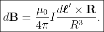
Because

ˆ R- R = R ,

(10)

an equivalent form is

|------------′------| | μ0- dℓ-×-R-- | dB = 4πI R3 . | --------------------

(11)

The two forms are identical.

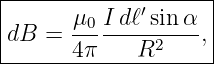
The magnitude is

|-------------′------| |dB = μ0-I-dℓ-sin-α-,| -------4π----R2------|

(12)

where α is the angle between dℓ′ and R.

Several features should be read directly from the equation:

the contribution is proportional to current I;
it is proportional to source-element length dℓ′;
it depends on orientation through sin α;
it decreases with source-to-observer distance;
its direction is set by the cross product dℓ′×R.

4 Direction from the right-hand rule

The direction of dB is perpendicular to the plane containing dℓ′ and R.

For a positive conventional current direction:

point the fingers of the right hand along dℓ′;
curl toward R through the smaller angle;
the thumb indicates the direction of dℓ′× R.

For a long straight wire, this local rule produces magnetic-field lines that circle the wire.

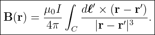
5 Integrating over a thin wire

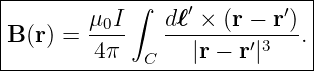
A complete wire contains many current elements, so the total field is the vector sum

|-----------∫-----′--------′--| B (r) = μ0I- d-ℓ-×-(r −-r). | | 4π C |r − r′|3 | -------------------------------

(13)

The path C follows the current-carrying wire.

This integral is a source integral. The observation position r is held fixed while the source coordinate r′ runs along the current path.

6 Example 1: direction from one current element

Suppose

dℓ′ = dℓ ˆx

(14)

and the observation point lies directly in the +y direction from the element, so

Rˆ = ˆy.

(15)

Then

dℓ′ × Rˆ = dℓ ˆx × ˆy = dℓ ˆz.

(16)

Therefore,

|-------------------------------| dB--points-in-the--+-z-direction.--

(17)

If the observation point were instead directly in the +x direction from the element, then dℓ′ and R would be parallel and

dB = 0

(18)

for that individual element.

7 The magnetic field of an infinitely long straight wire

Consider a straight wire along the z axis carrying current I in the +z direction. Let the observation point be a perpendicular distance s from the wire.

Symmetry tells us that the magnetic field must circle the wire. Its magnitude can depend only on s.

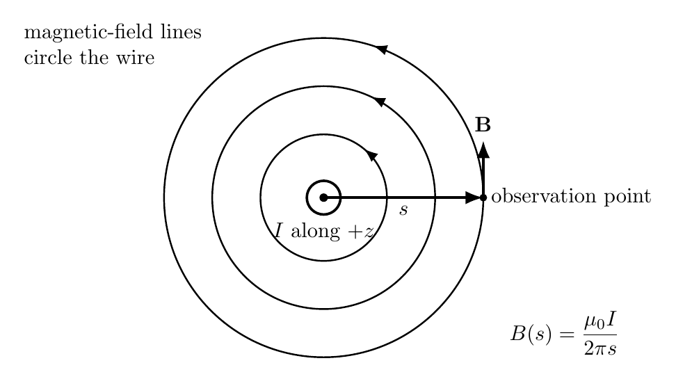
Figure. A long straight current produces circular magnetic-field lines. The right-hand rule sets their direction.

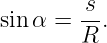
Choose a source element at coordinate z′. Its distance to the observation point is

√ -------- R = s2 + z′2.

(19)

The perpendicular factor in the cross product contributes

sin α = -s. R

(20)

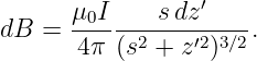
Therefore the field magnitude contributed in the azimuthal direction is

μ0I----s-dz′--- dB = 4π (s2 + z′2)3∕2.

(21)

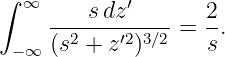
Integrating from z′ = −∞ to +∞,

μ0I ∫ ∞ s dz′ B (s) = ---- --2----′2-3∕2-. 4 π −∞ (s + z )

(22)

The integral evaluates to

∫ ∞ ′ ---s-dz-----= 2. −∞ (s2 + z′2)3∕2 s

(23)

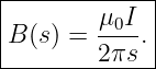
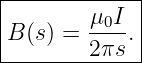
Hence

|------------| | μ0I- | B (s) = 2πs .| --------------

(24)

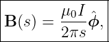
The vector field is

|--------------| |B (s) = μ0Iϕˆ, | ---------2πs----

(25)

where ϕ is the azimuthal direction around the wire.

This 1∕s dependence is an important result: the field of an ideal infinite line current does not fall as 1∕s².

8 Example 2: field near a straight wire

A long wire carries

I = 4.0A.

(26)

Find the magnetic-field magnitude at

s = 5.0cm = 0.050 m.

(27)

Using

μ0I B = ----, 2πs

(28)

we obtain

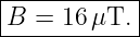
B	=	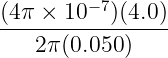(29)
	= 1.6 × 10⁻⁵ T.	(30)

Therefore,

|------------| |B = 16 μT. | -------------

(31)

The direction is tangent to the circular field line around the wire and is determined by the right-hand rule.

9 A finite straight wire

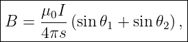
For a finite straight segment, the Biot–Savart integral gives

|-------------------------| | μ0I- | B = 4πs (sin𝜃1 + sin𝜃2), | ---------------------------

(32)

where s is the perpendicular distance from the observation point to the line containing the wire, and 𝜃₁ and 𝜃₂ are the endpoint angles measured from the perpendicular to the wire.

For an infinitely long wire,

𝜃 = 𝜃 = 90∘, 1 2

(33)

sin 𝜃1 + sin 𝜃2 = 2,

(34)

and the infinite-wire result is recovered.

10 Example 3: finite straight wire

A straight wire carries I = 3.0 A. An observation point lies s = 0.10 m from the wire, and the two endpoint angles are

𝜃1 = 𝜃2 = 45∘.

(35)

Then

B	=	(36)
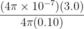	=	(37)
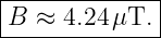
	≈ 4.24 × 10⁻⁶ T.	(38)

Thus

|-------------| B--≈-4.24μT.---

(39)

11 Field at the center of a circular current loop

Now consider a circular loop of radius a carrying current I.

At the center of the loop, every source element is the same distance

R = a

(40)

from the observation point, and each current element is perpendicular to R:

sin α = 1.

(41)

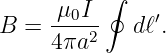
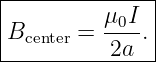
Therefore,

μ0-I dℓ′ dB = 4π a2 .

(42)

All contributions point along the same axis normal to the loop, so the magnitudes add directly:

∮ B = μ0I-- d ℓ′. 4πa2

(43)

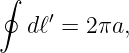
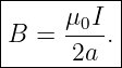
Because the circumference is

∮ dℓ′ = 2πa,

(44)

we obtain

|--------------| | μ0I | |Bcenter = ----.| -----------2a--

(45)

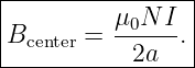
For N closely spaced turns,

|----------------| | μ0N-I- | |Bcenter = 2a .| -----------------

(46)

12 Magnetic field on the axis of a circular loop

The center result is a special case of the field anywhere on the loop axis.

Let the loop lie in the xy plane with radius a, and let the observation point lie on the z axis a distance z from the center.

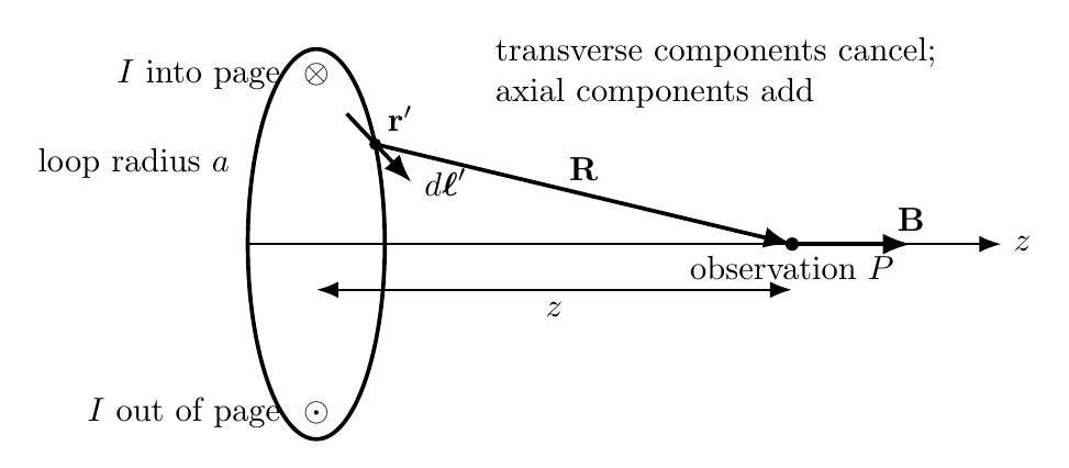
Figure. A circular current loop and an observation point on its axis. Transverse contributions from opposite current elements cancel, while axial components add.

Every source point on the loop is the same distance

√------- R = a2 + z2

(47)

from the observation point.

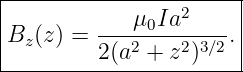
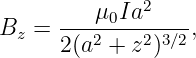
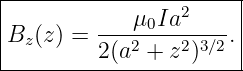
By symmetry, the components perpendicular to the z axis cancel around the loop. Only the axial components survive. Carrying out the Biot–Savart integral gives

|----------------2-----| |Bz(z) = ----μ0Ia-----.| ---------2-(a2-+-z2)3∕2--

(48)

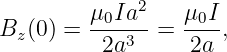
At z = 0,

μ0Ia2- μ0I- Bz(0) = 2a3 = 2a ,

(49)

as expected.

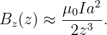
Far from the loop, where z ≫ a,

μ Ia2 Bz (z) ≈ -0----. 2z3

(50)

Thus the far magnetostatic field of a small current loop decreases approximately as 1∕z³ along its axis. This is the characteristic scaling of a magnetic dipole field, not the 1∕r scaling of a radiated far field from a time-varying antenna.

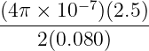
13 Example 4: field at the center of a loop

A single circular loop has

a = 0.080 m, I = 2.5 A.

(51)

Then

B	=	(52)
	=	(53)
	≈ 1.96 × 10⁻⁵ T.	(54)

Therefore,

|-------------| B--≈-19.6μT.---

(55)

14 Example 5: field on the loop axis

For the same loop, evaluate the field at

z = 0.060 m.

(56)

Using

μ Ia2 Bz = -----0------, 2(a2 + z2)3∕2

(57)

with a = 0.080 m and I = 2.5 A,

a² + z²	= (0.080)² + (0.060)²	(58)
	= 0.0100 m²,	(59)

2 2 3∕2 3 (a + z ) = 0.00100 m .

(60)

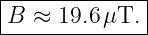
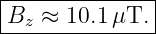
Hence

B_z	=	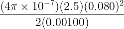(61)
	≈ 1.01 × 10⁻⁵ T.	(62)

Thus

|--------------| |Bz ≈ 10.1 μT. | ---------------

(63)

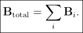
15 Superposition of magnetic fields

The Biot–Savart law is linear in current. Therefore magnetic fields from separate current distributions add vectorially:

|----------------| |B = ∑ B .| | total i | -----------i-----

(64)

This principle is essential for coils, paired Conductors, transmission structures, and arrays of current elements.

16 Example 6: two parallel wires

Two infinitely long parallel wires are separated by

d = 0.20 m

(65)

and each carries

I = 5.0A

(66)

in the same direction.

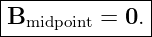
At the midpoint, the distance to either wire is

s = 0.10 m.

(67)

Each wire produces the same field magnitude,

B = μ0I-. 2πs

(68)

But the right-hand rule shows that the two field directions at the midpoint are opposite. Therefore,

|--------------| -Bmidpoint =-0.|

(69)

If one current is reversed, the two fields point in the same direction at the midpoint and add instead.

17 From a thin wire to a volume current density

EM08 introduced the current-density field J(r′). A small source volume dV ′ carrying current density behaves like a distributed current source.

The Biot–Savart law generalizes to

|-----------∫-----′---------′------| | μ0- J(r-) ×-(r-−-r-) ′ | |B (r) = 4π V |r − r′|3 dV .| -----------------------------------

(70)

This equation is structurally important. It has the form

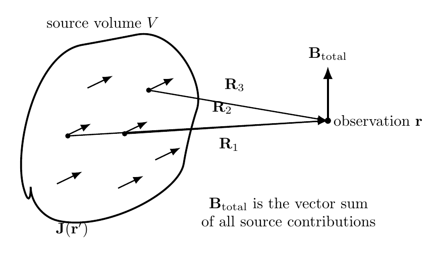
|---------------------------∫----------------------------------------------| |field at observation point = source contribution from every source point.| ---------------------------------------------------------------------------|

(71)

Figure. A distributed current is decomposed into many source elements. Their vector magnetic-field contributions are summed at the observation point.

This source-integration viewpoint will later become central in antenna theory. There, however, the source currents vary with time and propagation delay cannot be ignored.

18 Example 7: setting up a current-density source integral

Suppose a finite conductor occupies a source volume V and has known current density

J(r′).

(72)

At observation point r, the correct magnetostatic field integral is

μ0 ∫ ′ r − r′ ′ B(r) = --- J(r) × ------′3 dV . 4 π V |r − r|

(73)

Three roles must remain distinct:

r′ locates each source element;
r is the fixed observation point;
r − r′ points from source to observation.

This bookkeeping is exactly the same kind of source/observation distinction introduced for Coulomb fields in EM05.

19 Comparison with electric-field source integrals

For a static charge density,

∫ --1-- ′ -r −-r′- ′ E (r) = 4π𝜖 ρ(r )|r − r′|3 dV . 0 V

(74)

For a steady current density,

μ ∫ r − r′ B(r) = --0 J(r′) × ------′3 dV ′. 4 π V |r − r|

(75)

Both are source integrals with inverse-distance geometry, but the magnetic field includes a cross product with the current direction. Consequently magnetic-field direction is inherently tied to orientation and handedness.

20 Magnetostatic assumptions and the antenna warning

The Biot–Savart law used in this article assumes steady currents. This means

∂-ρ = 0 ∂t

(76)

and, consistently with the continuity equation,

∇ ⋅ J = 0

(77)

for the steady current distribution under consideration.

A radio antenna does not generally satisfy the steady-current assumption. Its charge and current distributions oscillate in time. Changes at the source do not influence distant points instantaneously; electromagnetic effects propagate at finite speed.

Therefore,

|------------------------------------------------------------| magnetostatic--Biot–Savart-⁄=-complete--antenna-radiation-law.-

(78)

The magnetostatic theory remains essential because it teaches the source-integration geometry and gives the correct low-frequency or quasi-static limit. Later articles will add Faraday induction, Maxwell’s correction, retarded fields, and electromagnetic-wave propagation.

21 Common misconceptions

The Biot–Savart direction is not generally along R. It is set by dℓ′× R.
The source coordinate and observation coordinate are different objects. r′ is integrated over; r is held fixed.
A current element parallel to R gives zero contribution at that observation point.
The field of an infinite straight wire falls as 1∕s, not 1∕s².
A small steady current loop has a magnetostatic dipole field that falls much faster than a radiated far field.
Magnetic fields add vectorially. Equal magnitudes do not guarantee reinforcement; directions can cause cancellation.
The magnetostatic Biot–Savart law is not sufficient by itself for a time-varying RF antenna.

22 Why this matters for antennas and RF

Antenna theory ultimately asks how distributed, time-varying currents and charges produce electromagnetic fields in space. The full answer requires time-dependent Maxwell theory, but EM11 establishes several pieces that survive into that more advanced treatment:

source point r′ versus observation point r;
separation vector R = r − r′;
decomposition of a distributed current into differential source elements;
vector superposition at the observation point;
cross-product geometry linking current orientation to field direction;
the idea that field calculations are integrals over source distributions.

These ideas will reappear later in Huygens-type aperture integrals, current-element radiation, phased arrays, and receive-aperture theory.

23 Summary

For a steady thin-wire current,

|-------------------| | μ0 dℓ′ × R | dB = --I ----3--. | -------4π----R------

(79)

The total field is

|-----------∫-----------------| | μ0I d ℓ′ × (r − r′) | B (r) = ---- --------′-3--. | ---------4π--C----|r −-r-|-----

(80)

For an infinitely long straight wire,

|------------| | μ0I- | B-(s)-=-2πs-.-

(81)

At the center of a circular loop,

|-----μ-I--| |B = -0--.| -------2a--|

(82)

On the loop axis,

|----------------2-----| |Bz(z) = ----μ0Ia-----.| | 2 (a2 + z2)3∕2 | ------------------------

(83)

For a volume current density,

|----------------------------------| | μ ∫ J(r′) × (r − r′) | |B (r) = -0- ---------------dV ′.| ---------4π--V-----|r-−-r′|3---------

(84)

EM11 therefore establishes the magnetostatic source-field integral machinery. The next stage can introduce the integral and differential relationships between current and magnetic-field circulation before the series moves into time-varying induction and Maxwell’s equations.

References

[1] David J. Griffiths, Introduction to Electrodynamics, 4th ed., Cambridge University Press, 2017.

[2] Edward M. Purcell and David J. Morin, Electricity and Magnetism, 3rd ed., Cambridge University Press, 2013.

[3] Samuel J. Ling, Jeff Sanny, and William Moebs, University Physics, Volume 2, OpenStax, 2016, sections on magnetic fields produced by currents and the Biot–Savart law.

[4] Richard P. Feynman, Robert B. Leighton, and Matthew Sands, The Feynman Lectures on Physics, Volume II, Addison-Wesley, 1964, chapters on steady currents and magnetic fields.

[5] Massachusetts Institute of Technology, 8.02 Physics II: Electricity and Magnetism, MIT OpenCourseWare, materials on Biot–Savart law, current elements, straight wires, and loops.

"Electromagnetic Waves: Magnetic Fields Produced by Currents" is owned by bloftin.
(view preamble)