|
|
|
|||||||
The receive antenna gain and system noise temperature are assumed to be referred consistently to the same receiver input reference plane. This is essential: a feed loss, radome loss, or mismatch loss must not be subtracted again if its effect has already been absorbed into the quoted G∕T or Tsys.
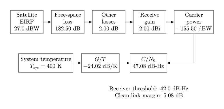
Figure. End-to-end GNSS-style link chain used in this worked example. The desired carrier and receiver noise quantities are kept at consistent reference planes.
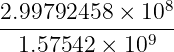
2. Frequency, wavelength, and geometryThe wavelength is
where
Thus
So the L1-like carrier wavelength is about 19.0 cm. The range r = 20,200 km is used here as a simple GNSS-scale slant range for the worked calculation. In a real receiver the instantaneous satellite-to-user slant range varies with satellite elevation and user geometry.
3. Satellite EIRPEquivalent isotropically radiated power is the product of transmitter power and transmit antenna gain, after losses ahead of the antenna have been accounted for:
in linear units, or
in decibel form. For this example the satellite directional EIRP toward the user is already given:
The corresponding isotropic-equivalent linear power is
This does not mean that the transmitter necessarily dissipates 501 W of RF power. EIRP includes antenna directivity and represents the isotropic transmitter power that would create the same far-field power density in the specified direction.
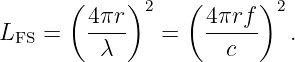
4. Free-space path lossFrom the Friis relation, free-space path loss is
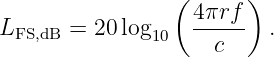
In decibels,
Substitution gives
Hence
The linear path-loss ratio is enormous:
This is geometric spreading and receive-aperture scaling, not absorption of energy by empty space.
5. Received carrier powerThe received carrier power at the chosen receiver reference plane is
Therefore
Thus
In dBm,
In watts,
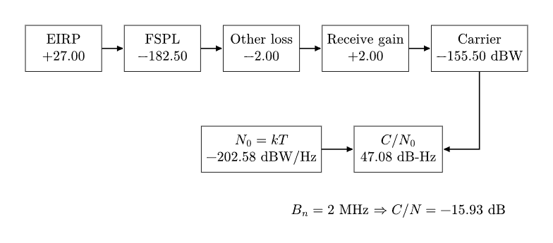
Figure. The same link written as additive dB bookkeeping. Once the carrier reaches the receiver reference plane, it is compared with the receiver noise spectral density.
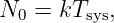
6. Receiver thermal-noise densityFor system noise temperature Tsys, the available thermal-noise power spectral density is
where
At Tsys = 400 K,
In logarithmic units,
Therefore
7. Receiver G∕TThe receiver figure of merit is
For the assumed receive antenna and system temperature,
Thus
8. Carrier-to-noise-density ratio C∕N0There are two useful ways to calculate C∕N0. Performing both provides an excellent consistency check.
8.1 Method A: carrier power minus noise densityBecause carrier power is in dBW and noise density is in dBW/Hz,
Hence
Therefore
8.2 Method B: the end-to-end G∕T equationUsing the complete link-budget relation,
Substitution gives
exactly matching Method A to rounding. In linear units,
The unit “Hz” appears because a power is divided by a power spectral density.
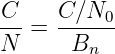
9. From C∕N0 to finite-bandwidth C∕NFor an ideal equivalent noise bandwidth Bn,
Therefore
and in decibels,
For Bn = 2.00 MHz,
so
Thus
The corresponding total thermal noise power is
or
This is substantially larger than the carrier power, which is Normal for spread-spectrum GNSS reception before correlation and signal processing.
10. Required threshold and clean-link marginAssume this particular receiver requires
for the operating mode under consideration. This value is a receiver-design assumption, not a universal GNSS constant. The clean-link margin is
Therefore
At 2 MHz the same threshold would correspond to
The difference between the clean C∕N = −15.93 dB and the threshold-equivalent C∕N = −21.01 dB is again 5.08 dB, as expected.
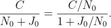
11. Allowable additive interference densityNow suppose an admitted interferer can be modeled as additional uncorrelated, noise-like spectral density J0 at the same receiver reference plane. The effective carrier-to-disturbance density becomes
Factor out N0:
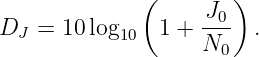
Thus the interference-induced degradation is
At the allowable limit, the interference consumes the entire clean-link margin:
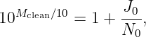
Therefore
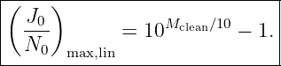
which yields
Using Mclean = 5.076 dB,
In decibels,
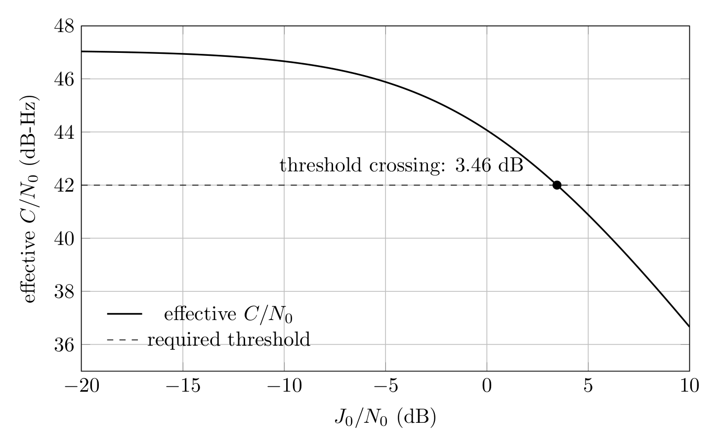
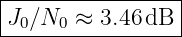
This is the maximum additive noise-like interference-density ratio permitted by the assumed 42 dB-Hz threshold and the nominal clean link.
Figure. Effective C∕N0 as additive noise-like interference increases. The assumed 42 dB-Hz requirement is reached at J0∕N0 ≈ 3.46 dB.
12. Convert the allowable interference to absolute unitsBecause
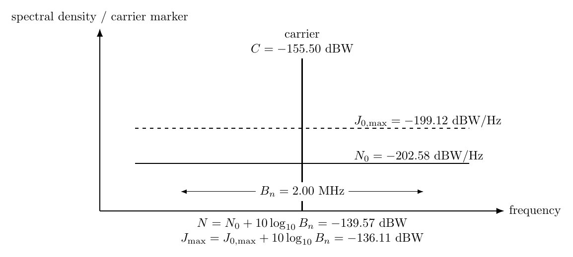
the maximum admitted interference density is
Therefore
If the same noise-like density occupies the full 2.00 MHz receiver noise bandwidth, the admitted in-band interference power is
Thus
Figure. Noise and allowable interference shown as spectral densities and as integrated powers over the 2 MHz equivalent noise bandwidth.
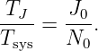
13. Equivalent interference temperatureBecause thermal-noise density is N0 = kTsys, a noise-like interference density can be represented by an equivalent temperature
Using the ratio form is simpler:
At the allowable limit,
The effective disturbance temperature is then
The large temperature value does not imply that the physical receiver is at 1287 K; it is an equivalent noise-temperature representation of the admitted interference.
14. Why allowable J∕S can be positiveIn a GNSS link it is common for the desired spread-spectrum carrier to be below the total wideband thermal-noise power before correlation. The same can be true relative to admitted broadband interference. At the interference limit,
while
Therefore
Thus
at the same point where the effective C∕N0 has only fallen from 47.08 to 42.0 dB-Hz. This is not a contradiction. J∕S compares integrated powers, while degradation in this model is governed by the ratio of interference spectral density to thermal-noise spectral density. Bandwidth, spectral overlap, receiver filtering, correlation properties, front-end linearity, and signal structure matter. Consequently, J∕S alone is not a universal predictor of GNSS receiver performance [2].
15. Compact end-to-end budget table
16. Sensitivity rules worth rememberingThe completed budget makes several useful one-line sensitivity rules visible:
These rules are useful for rapid link-budget sanity checks, but they do not replace careful reference-plane bookkeeping.
17. Scope of the interference calculationThe interference result in this example is intentionally restricted to an additive, uncorrelated, noise-like disturbance that is admitted through the receiver bandwidth without causing front-end saturation or nonlinear behavior. Narrowband continuous-wave interference, swept interference, pulsed interference, signals with strong spectral structure, AGC effects, quantizer overload, intermodulation, correlator effects, and antenna-array spatial rejection require more detailed models. In those cases the scalar J0∕N0 calculation here remains a useful baseline, but it is not sufficient by itself.
18. Julia numerical checkThe companion file EM28E2_gnss_link_budget_check.jl reproduces the complete chain numerically and verifies the threshold-crossing value of J0∕N0. It also evaluates the effective C∕N0 over a sweep of interference-density ratios for comparison with the final figure.
SummaryBeginning with a directional satellite EIRP of 27.0 dBW, an L1-like 20,200 km free-space link gives
After 2.0 dB of other losses and 2.0 dBi of receive gain, the received carrier is
For Tsys = 400 K,
and therefore
Across 2 MHz,
For an illustrative 42.0 dB-Hz receiver requirement, the clean margin is 5.08 dB. Under the additive noise-like interference model, this allows
before the threshold is reached.
References
References
[1] E. D. Kaplan and C. J. Hegarty, editors, Understanding GPS/GNSS: Principles and Applications, 3rd ed., Artech House, 2017. [2] J. W. Betz, Engineering Satellite-Based Navigation and Timing: Global Navigation Satellite Systems, Signals, and Receivers, Wiley-IEEE Press, 2016. [3] D. M. Pozar, Microwave Engineering, 4th ed., Wiley, 2012. [4] C. A. Balanis, Antenna Theory: Analysis and Design, 4th ed., Wiley, 2016. "Electromagnetic Waves, Antennas, and RF: Detailed GNSS Link-Budget Example from Satellite EIRP to Interference Margin" is owned by bloftin.
This object's parent. Cross-references: scalar, representation, clean-link margin, Normal, thermal noise power, equivalent noise bandwidth, temperature, system, energy, free-space path loss, relation, antenna directivity, units, equivalent isotropically radiated power, system noise temperature, antenna gain, noise temperature, carrier frequency, Power This is version 1 of Electromagnetic Waves, Antennas, and RF: Detailed GNSS Link-Budget Example from Satellite EIRP to Interference Margin, born on 2026-10-10. Object id is 1463, canonical name is ElectromagneticWavesAntennasAndRFDetailedGNSSLinkBudgetExampleFromSatelliteEIRPToInterferenceMargin. Accessed 1 times total. Classification:
|
|
|
|
Pending Errata and AddendaNone.
|
DiscussionNo messages.
|
Interact |
![[parent]](https://images.physicslibrary.org/images/uparrow.png)
 req
req





![[4π (20.2 × 10⁶)(1.57542 × 10⁹ )]
----------------------8-------
2.99792458 × 10](https://images.physicslibrary.org/cache/objects/1463/make4ht/ElectromagneticWavesAntennasAndRFDetailedGNSSLinkBudgetExampleFromSatelliteEIRPToInterferenceMargin10x.png)




















 clean
clean  req
req