Electromagnetic Waves, Antennas, and RF: RF Interference and Jamming, J∕S, J∕N0,
C∕(N + J), and Receiver Degradation
EM25 determined how much desired RF Power reaches a receiver. EM26 then compared that
desired carrier power with thermal-noise density through C∕N0. Real receivers must also operate in
the presence of other radio-frequency signals. These may be unintended cochannel emissions,
adjacent-channel leakage, harmonics, spurious radiation, or deliberate jamming. The same
received-power bookkeeping applies in each case; what changes is the physical source and, often,
the spectral structure of the interference [1, 2, 4, 5].
This article develops receiver-side interference metrics for analysis and robustness studies. The
central chain is
The most important conceptual point is that interference power, thermal-noise density, and signal
power are different kinds of quantities. They can be combined only after they have been referred to
a common receiver reference plane and, when necessary, integrated over the same effective
bandwidth.
1 Notation and receiver reference plane
Let
- S denote the desired received signal power;
- C denote the desired received carrier or signal power when using the conventional
C∕N0 notation;
- J denote received interference power after the relevant propagation and antenna effects;
- N0 = kTsys denote thermal-noise power spectral density;
- N = N0Bn denote thermal-noise power in receiver equivalent noise bandwidth Bn;
- J0 denote an equivalent interference power spectral density when a density model is
appropriate.
For the power-ratio derivations below, S and C may refer to the same desired received
RF power. The letter C is retained where the conventional carrier-to-noise notation is
useful.
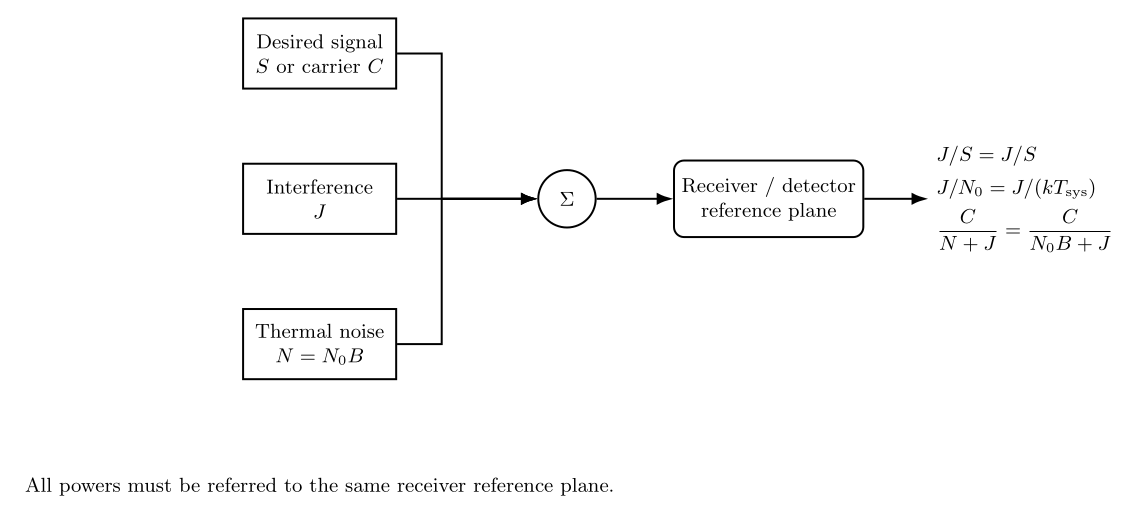
Figure. Desired signal, interference, and thermal noise must be referred to the same
receiver reference plane before forming J∕S, J∕N0, or C∕(N + J).
The basic quantities have different dimensions:
| Quantity | Linear units | Common logarithmic units |
|
|
|
| J∕S | dimensionless | dB |
| J∕N0 | Hz | dB-Hz |
| J0∕N0 | dimensionless | dB |
| C∕(N + J) | dimensionless | dB |
This distinction prevents one of the most common errors in interference analysis: adding or
subtracting a total power directly from a spectral density without first accounting for
bandwidth.
2 Jam- or interference-to-signal ratio J∕S
At a specified receiver reference plane,
In decibels,
If S = C, then the same ratio may be written J∕C.
A negative J∕S means the interference power is below the desired-signal power. A positive J∕S
means the interference power is above it. Neither case, by itself, predicts receiver failure. Receiver
performance also depends on thermal noise, bandwidth, spectral overlap, modulation,
coding, filtering, correlation processing, front-end linearity, and other implementation
details.
Worked example: received-power ratio
Suppose
Then
 dB dB | = −136 − (−130) | (5)
|
| = −6 dB. | (6) |
Therefore
In linear form,
Thus the interference power is about 25.1% of the desired received power.
3 A second RF link produces the received interference power
EM25 showed that a desired transmitter produces received power through its own link budget.
An interfering transmitter obeys the same propagation physics. For two independent
links,
| SdBW | = EIRPS,dBW − LS,path − LS,other + Gr(ΩS), | (9)
|
| JdBW | = EIRPJ,dBW − LJ,path − LJ,other + Gr(ΩJ). | (10) |
The receive-antenna gain can differ because the desired signal and the interfering signal may
arrive from different directions. Their polarizations and frequencies may also differ,
in which case the corresponding mismatch and propagation terms must be included
separately.
Subtracting the two received-power equations gives
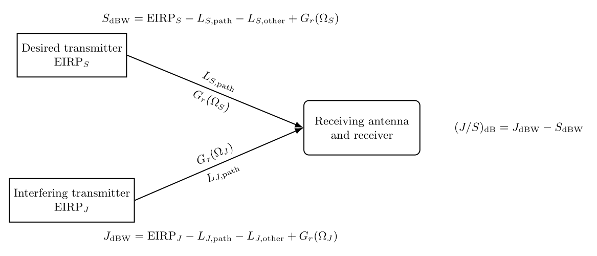
Figure. A desired signal and an interfering signal are separate RF links that terminate at
the same receiver. Antenna directionality, propagation loss, and other losses act
independently on the two paths.
This formulation is particularly useful for receiver susceptibility studies because it separates
transmitter, path, and receive-antenna effects without requiring the two sources to share the same
geometry.
4 Interference-to-noise-density ratio J∕N0
EM26 defined
The ratio of a total received interference power J to thermal-noise density is therefore
Because J has units W while N0 has units W/Hz,
Consequently J∕N0 is conventionally reported in dB-Hz:
Worked example: J∕N0 from system temperature
Let
and let the received interference power be
The noise density is
| N0,dBW∕Hz | = 10 log 10(kTsys) | (18)
|
| ≈−203.16 dBW/Hz. | (19) |
Hence
 dB−Hz dB−Hz | = −150 − (−203.16) | (20)
|
| = 53.16 dB-Hz. | (21) |
Thus
5 Connecting J∕S, J∕N0, and C∕N0
If S = C and all quantities are referred to the same plane and the same thermal-noise density N0,
then
Therefore
In logarithmic units,
The dB-Hz units cancel in the subtraction, leaving a dimensionless power ratio in dB.
6 Bandwidth converts J∕N0 into J∕N
Thermal-noise power in equivalent noise bandwidth Bn is
Hence
Thus
In decibels,
This is why J∕N0 and J∕N answer different questions. J∕N0 compares an integrated interference
power with a noise density. J∕N compares interference power with the actual thermal-noise power
admitted by a specified bandwidth.
7 Spectral overlap: the receiver only admits part of the interference
A total transmitter or antenna-terminal interference power is not automatically the interference
power that reaches the detector. Let SJ(f) denote the interference power spectral density at the
receiver input and let H(f) denote the receiver transfer function. The admitted interference power
is
Similarly, for flat thermal-noise density N0,
If |H(f)|2 is normalized to unity at its peak, define the equivalent noise bandwidth
Then
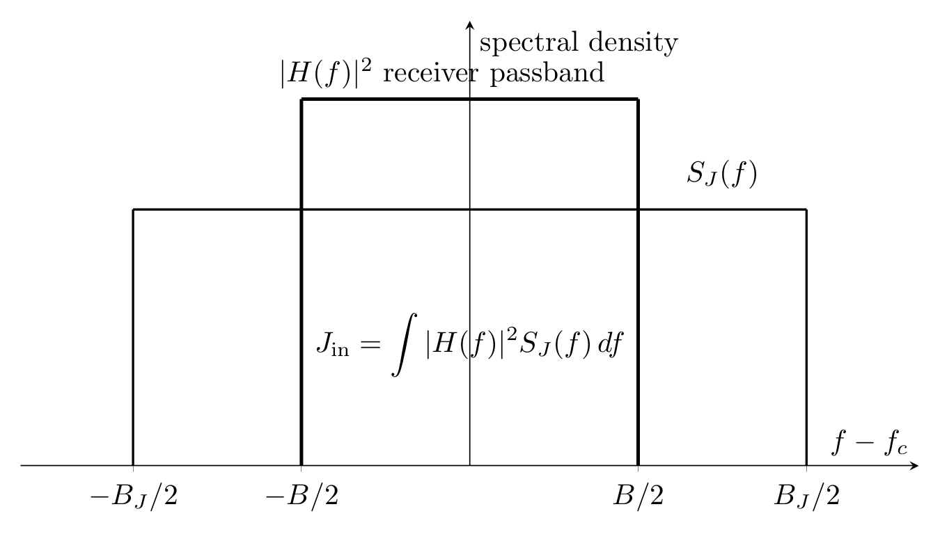
Figure. Interference degradation depends on the spectral overlap between the interfering
spectrum SJ(f) and the receiver transfer function H(f), not merely on total emitted or
incident power.
If a noise-like interferer is approximately flat with density J0 throughout the receiver passband,
then
This special case permits especially simple density-ratio formulas.
8 Deriving C∕(N + J)
Suppose the detector sees desired carrier power C, thermal-noise power N, and admitted
interference power J. If the interference contribution may be treated as an additive
uncorrelated power for the receiver metric of interest, then the total undesired power
is
The resulting carrier-to-noise-plus-interference ratio is
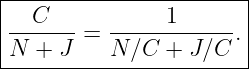
Divide numerator and denominator by C:
Alternatively, factor out N:
Thus
This equation gives the receiver degradation caused by additive in-band interference.
9 Receiver degradation factor
Define the degradation factor as the ratio of the noise-only carrier-to-noise ratio to the
carrier-to-noise-plus-interference ratio:
Substituting the result above,
In decibels,
This is a positive penalty. It is the number of decibels by which C∕(N + J) lies below the
noise-only C∕N.
Three useful landmarks are
| J∕N = −10 dB |  D ≈ 0.414 dB, D ≈ 0.414 dB, | (45)
|
| J∕N = 0 dB |  D = 3.010 dB, D = 3.010 dB, | (46)
|
| J∕N = +10 dB |  D ≈ 10.414 dB. D ≈ 10.414 dB. | (47) |
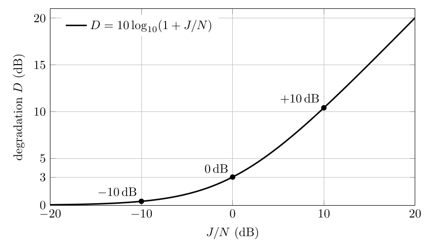
Figure. Additive-power degradation D = 10 log 10(1 + J∕N). Equal interference and
thermal-noise powers produce a 3.01 dB penalty.
10 Using C∕N0 and J∕N0 directly
EM26 often provides C∕N0 rather than C∕N. Since
we may write
Therefore
The numerator and denominator on the right both have units of hertz, so the final ratio is
dimensionless.
Worked example: C∕N0, J∕N0, and finite bandwidth
Suppose
First compute the noise-only value:
| (C∕N)dB | = 60 − 10 log 10(105) | (53)
|
| = 60 − 50 | (54)
|
| = 10 dB. | (55) |
Next,
| (J∕N)dB | = 55 − 50 | (56)
|
| = 5 dB. | (57) |
Thus
The degradation is
| DdB | = 10 log 10(1 + 3.162) | (59)
|
| = 6.19 dB. | (60) |
Therefore
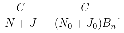
11 Noise-like interference density J0
For broadband noise-like interference that is approximately flat across the receiver passband,
Then
| N + J | = N0Bn + J0Bn | (63)
|
| = (N0 + J0)Bn. | (64) |
Hence
It is often convenient to define the effective carrier-to-noise-plus-interference density
ratio
Relative to the thermal-noise-only value,
 | =  . . | (67) |
Therefore the density-domain degradation is
Worked example: interference density below thermal noise density
Let
Then
The degradation is
| DdB | = 10 log 10(1 + 0.2512) | (71)
|
| ≈ 0.973 dB. | (72) |
Thus even an interference density 6 dB below thermal-noise density raises the combined
noise-plus-interference floor by almost 1 dB.
If the original
then
12 Equivalent interference temperature
Noise-like interference can also be represented by an equivalent temperature. If in-band
interference power is J in bandwidth Bn, define
Since
we may write
| N + J | = kTsysBn + kTJBn | (77)
|
| = k(Tsys + TJ)Bn. | (78) |
Therefore
for the special case in which the interference is legitimately represented as additive noise over the
bandwidth of interest.
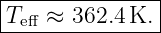
Worked example: equivalent interference temperature
Suppose
is admitted over
Then
| TJ | =  | (82)
|
| ≈ 72.4 K. | (83) |
For a 290 K receiver system,
The associated degradation is
| DdB | = 10 log 10 | (85)
|
| ≈ 0.97 dB. | (86) |
This is the same result obtained from 1 + J∕N.
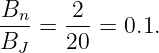
13 Worked example: broadband spectral overlap
Suppose a cochannel noise-like interferer has total received power
spread uniformly across
Assume an ideal rectangular receiver bandwidth
lies entirely inside the interference band. The admitted fraction is
Therefore
| Jin,dBm | = −90 + 10 log 10(0.1) | (91)
|
| = −100 dBm. | (92) |
At 290 K,
| NdBm | = −173.98 + 10 log 10(2 × 10⁶) | (93)
|
| ≈−110.96 dBm. | (94) |
Hence
The degradation is
This calculation demonstrates why total interference power without bandwidth information can be
misleading. The receiver responds to the portion of the interference spectrum that survives its
transfer function.
14 Worked example: a GNSS-style receiver-side calculation
Consider an illustrative received carrier power
and system noise temperature
From EM26,
so
Now suppose the receiver input contains an interfering signal with total admitted power
Then
and
If one models this interference simply as additive in-band power over
then
| (C∕N)dB | = 44.08 − 10 log 10(2 × 10⁶) | (105)
|
| ≈−18.93 dB, | (106) |
while
The additive-power penalty is therefore only
Hence the scalar model gives
This result is intentionally instructive: a large J∕S does not uniquely determine receiver
degradation. In a spread-spectrum or correlation receiver, a narrowband, pulsed, swept, structured,
or partially correlated interferer may behave very differently from broadband Gaussian noise
having the same total power. Acquisition, tracking, automatic-gain-control behavior, and front-end
dynamic range require additional receiver-specific models [4, 5].
15 When C∕(N + J) is not enough
The equation
is an additive-power model. It is highly useful, but it does not describe every interference
mechanism. Several distinctions matter.
Narrowband versus broadband interference
A narrowband tone and broadband noise can have the same total received power J but produce
different detector behavior. The correct first step is always to calculate the admitted
interference
For modulation- or correlation-based receivers, the relevant transfer function may include more
than the analog RF filter.
In-band versus out-of-band interference
A signal outside the final channel bandwidth may contribute little directly to Jin after filtering.
Nevertheless, if it is sufficiently strong at an earlier receiver stage, it can affect automatic gain
control, amplifier compression, mixer products, or analog-to-digital-converter dynamic range.
These are nonlinear or implementation-dependent effects and cannot be predicted by the simple
additive N + J formula alone.
Deterministic versus noise-like interference
Thermal noise is stochastic and is naturally described by N0. A deterministic sinusoid is not
thermal noise. Representing it by an equivalent J0 is only appropriate when the receiver metric
averages its effect in a way that makes a density model meaningful.
Waveform correlation
A receiver designed to correlate against a known signal can strongly suppress some waveform
components and respond strongly to others. Consequently the same pre-correlation J∕S may
correspond to different post-correlation performance. A scalar link metric should therefore be
viewed as one layer of the analysis, not a complete receiver model.
16 A useful hierarchy of interference metrics
The different ratios answer different physical questions:
 | : How strong is received interference relative to the desired signal? | (112)
|
 | : How large is total interference relative to thermal-noise density? | (113)
|
 | : How large is admitted interference relative to in-band thermal noise? | (114)
|
 | : How large is noise-like interference density relative to thermal-noise density? |
(115)
|
 | : What additive carrier-to-undesired-power ratio remains at the chosen detector plane? |
(116) |
No single ratio replaces the others. The appropriate quantity depends on whether one is studying
RF propagation, spectral occupancy, front-end loading, demodulation, or a particular
tracking/detection process.
17 Summary
The desired-signal and interference powers are separate RF links that terminate at a common
receiver. At a common reference plane,
Thermal-noise density gives
with dB-Hz units, while finite bandwidth converts this to
The receiver admits interference according to
When the admitted interference may be treated as additive uncorrelated power,
and the degradation relative to thermal noise alone is
For flat noise-like interference,
EM27 therefore extends the EM25–EM26 link-budget chain to
The next article can combine the complete transmit, propagation, antenna, receiver-noise, and
interference models into a single end-to-end RF/ link budget.
References
[1] B. Sklar, Digital Communications: Fundamentals and Applications, 2nd ed., Prentice
Hall, 2001.
[2] D. M. Pozar, Microwave Engineering, 4th ed., Wiley, 2012.
[3] C. A. Balanis, Antenna Theory: Analysis and Design, 4th ed., Wiley, 2016.
[4] E. D. Kaplan and C. J. Hegarty, eds., Understanding GPS/GNSS: Principles and
Applications, 3rd ed., Artech House, 2017.
[5] J. W. Betz, Engineering Satellite-Based Navigation and Timing: Global Navigation
Satellite Systems, Signals, and Receivers, Wiley-IEEE Press, 2016.



![[ ]
-J- = Hz.
N0](https://images.physicslibrary.org/cache/objects/1459/make4ht/ElectromagneticWavesAntennasAndRFRFInterferenceAndJamming10x.png)