Electromagnetic Waves, Antennas, and RF: Thermal Noise, Noise Temperature, Noise Figure,
G∕T, and C∕N0
EM25 established how transmitted electromagnetic power becomes received carrier power. A useful
receiver, however, does not measure carrier power in isolation. It must distinguish the carrier from
random fluctuations generated by the antenna environment and by the receiver electronics
themselves.
The central chain in this article is
The objective is to derive the engineering quantities from thermal physics and power spectral
density rather than introduce them as isolated link-budget rules [2, 1, 3, 4, 5].
1 From received carrier power to detectability
Suppose EM25 predicts a received carrier power C at the receiver input. Whether that carrier is
useful depends on the competing noise power. If the receiver processes bandwidth B, then the
thermal-noise power is ultimately of the form
where k is Boltzmann’s constant and T is an appropriate noise temperature.
The appearance of B means that noise power depends on receiver bandwidth. Carrier power does
not acquire the same proportional dependence. This motivates a bandwidth-independent
comparison between carrier power and noise density:
Here N0 has units of W/Hz, so C∕N0 has units of hertz and is conventionally reported in
dB-Hz.
2 Thermal agitation and Johnson–Nyquist noise
A resistor at nonzero temperature contains charge carriers in continual thermal motion. Even when
the average current is zero, the instantaneous voltage fluctuates randomly. In the classical
low-frequency limit, the open-circuit voltage-noise power spectral density of a resistor R at
absolute temperature T is
Over an ideal bandwidth B in which R and T may be regarded as constant,
Thus the RMS open-circuit noise voltage is
The noise voltage is random; the expression above specifies its mean-square strength, not a
deterministic sinusoidal amplitude.
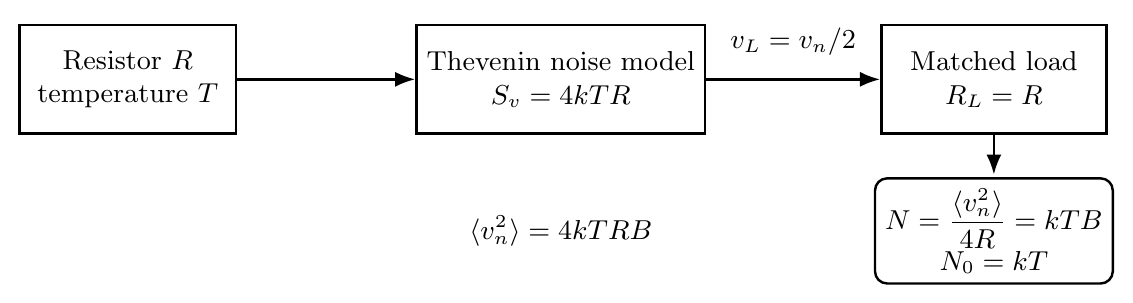
Figure. Johnson–Nyquist noise. A thermal resistor can be represented by a random
Thevenin voltage source. With a matched load, the available noise power becomes kTB.
3 Why a matched resistor delivers kTB
Model the noisy resistor as an ideal noiseless resistance R in series with a random source
having
Connect a matched load RL = R. The load receives half of the open-circuit voltage,
so
The average noise power delivered to the load is
Therefore
The resistance has disappeared. A matched resistor at temperature T makes the same available
thermal-noise power kTB regardless of its resistance value, within the assumptions of the classical
model.
4 Noise spectral density N0
If the available noise power in bandwidth B is
then the corresponding available noise-power spectral density is
The SI units are
Since one hertz is one inverse second, W/Hz is dimensionally equivalent to joules. In
communications engineering, however, W/Hz keeps the spectral-density interpretation
visible.
At the standard reference temperature
we have
| N0 | = kT0 | (17)
|
| = (1.380649 × 10⁻²³)(290) | (18)
|
| = 4.0039 × 10⁻²¹ W/Hz. | (19) |
In logarithmic units,
and therefore
The familiar “−174 dBm/Hz thermal-noise floor” is therefore a noise-density value near room
temperature, not the total noise power of a receiver.
For example, over B = 1 MHz,
so
5 Equivalent noise temperature
Noise temperature converts the noise produced by a component into the temperature of an
equivalent thermal source. If a noisy two-port contributes an equivalent input noise density N0,e,
define
The parameter Te does not necessarily equal the component’s physical temperature. It is an
equivalent input quantity that reproduces the component’s noise degradation.
If the source at the input has noise temperature Ts, an ideal noiseless gain G would produce
output noise
A real amplifier adds its own noise. Using equivalent input temperature Te,
6 Noise factor and noise figure
Noise factor compares the input and output signal-to-noise ratios:
For the standard reference source temperature T0 = 290 K,
Hence
Noise figure is the logarithmic form:
For example, if
then
and
7 Cascaded receiver noise: why the first stage matters
Consider cascaded stages with power gains G1,G2,… and noise factors F1,F2,…. Referred to the
input, the total noise factor is
Equivalently, in noise-temperature form,
These are often called the Friis cascade formulas for noise. They are distinct from the Friis
transmission equation of EM25, although both are historically associated with Harald
Friis.
The key physical lesson is that large first-stage gain suppresses the input-referred contribution of
later stages.
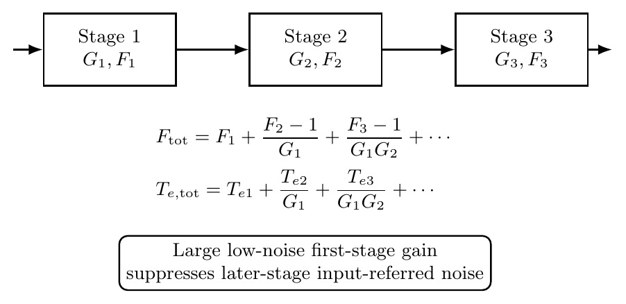
Figure. Cascaded receiver noise. Later-stage equivalent input noise is divided by the gain
preceding it, which is why low-noise amplification near the antenna is so valuable.
8 Passive loss before the LNA
A passive component with linear power loss L ≥ 1 has gain
At physical temperature Tp, its equivalent input noise temperature is
At the standard temperature T0, its noise factor is simply
This result explains a major receiver-design rule: loss before the first low-noise amplifier is
especially damaging. It attenuates the desired carrier before amplification and simultaneously
contributes thermal noise.
For a 1.0 dB cable loss,
At 290 K,
9 Antenna noise temperature
An antenna receives thermal electromagnetic radiation from the directions in its pattern. The
resulting available noise can be represented by an antenna noise temperature TA such
that
Conceptually, TA is a pattern-weighted measure of environmental brightness temperature. It can
depend on antenna pointing, frequency, ground pickup, atmosphere, sky background, and radome
or feed losses.
The antenna temperature need not equal the antenna’s physical temperature. A receiving
antenna pointed toward cold sky and the same antenna pointed toward warm ground can
have very different TA even though the metal structure itself is at the same physical
temperature.
10 System noise temperature
At a chosen receiver input reference plane, define the total system noise temperature
by
For a simple model in which antenna noise and receiver equivalent input noise are referred to the
same plane,
If feed loss lies between the antenna and LNA, its effect must be transformed to the same reference
plane rather than added blindly. The exact bookkeeping depends on where TA, gain, and received
carrier power are defined.
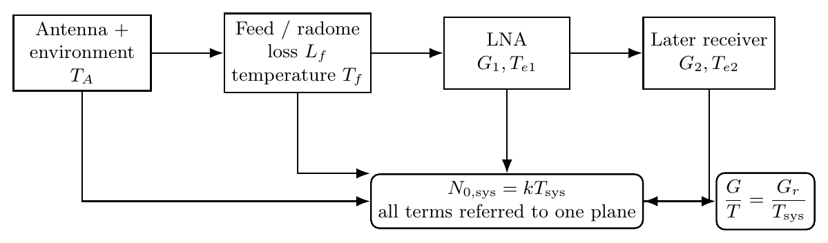
Figure. Receiver noise-temperature chain. Antenna/environment noise and receiver-added
noise are referred to a common input plane to form Tsys. The receiving gain divided by this
temperature forms G∕T.
11 The receiver figure of merit G∕T
Received carrier power improves with receive antenna gain Gr, while thermal-noise
density increases with system temperature Tsys. Their natural combined figure of merit
is
In logarithmic units,
For example, if
then
and
A higher G∕T means a stronger carrier relative to the receiver’s thermal-noise density.
12 Carrier-to-noise-density ratio C∕N0
Let the received carrier power at the chosen receiver reference plane be C. Since
we define
In decibel form,
Since
we may also write
This equation is one of the most important bridges between an RF link budget and receiver
performance.
13 Direct C∕N0 link-budget form
From EM25, the received carrier in dB form may be written schematically as
Substituting into the C∕N0 equation and grouping Gr with Tsys gives
This form makes the transmit and receive roles visually distinct:
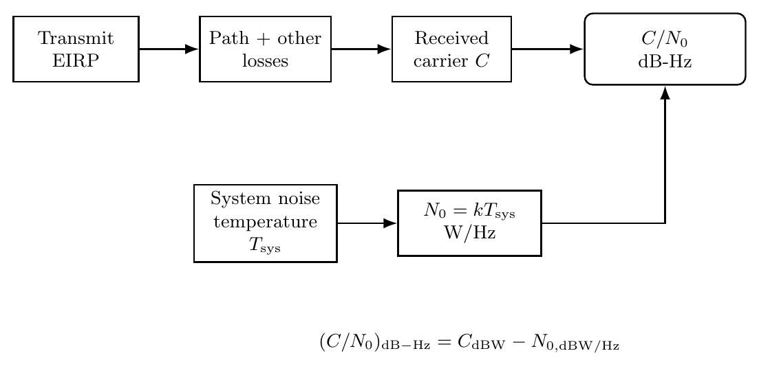
Figure. C∕N0 link-budget chain. EM25 supplies received carrier power; thermal physics
supplies N0 = kTsys; their ratio gives a bandwidth-independent carrier-quality metric.
14 Relationship between C∕N0 and C∕N
In a noise-equivalent bandwidth B,
Therefore
Hence
For example, if
and
then
This is not contradictory. A signal can have a useful spectral concentration or correlation structure
even when its total carrier power is below the integrated wideband thermal noise. Later
signal-processing articles can connect this idea to processing gain and Eb∕N0.
15 GNSS-style numerical example
EM25 used an illustrative L1-like link at
with received carrier power
Take an illustrative system noise temperature
Then
| N0 | = 10 log 10(kTsys) | (66)
|
| = −228.60 + 10 log 10(300) | (67)
|
| ≈−203.83 dBW/Hz. | (68) |
Therefore
 | = −157.50 − (−203.83) | (69)
|
| ≈ 46.33 dB-Hz. | (70) |
Thus
The purpose of this example is not to specify a particular GNSS satellite or receiver. It
demonstrates how an EM25 received-power result becomes a receiver-quality metric once Tsys is
known.
16 Classical approximation and quantum correction
The result N0 = kT is the classical limit. At sufficiently high frequency or sufficiently low
temperature, the available thermal-noise energy per mode is better represented by the Planck
factor
When
use
so
At ordinary RF and microwave frequencies near room temperature, the classical approximation is
usually excellent. The quantum correction becomes increasingly important for millimeter-wave,
submillimeter-wave, cryogenic, and quantum receiver systems.
17 Reference-plane discipline
Noise calculations are extremely sensitive to reference-plane ambiguity. Before combining
quantities, state explicitly:
- where carrier power C is defined;
- where antenna temperature TA is defined;
- whether feed loss is before or after that plane;
- whether antenna gain is realized gain or gain excluding mismatch;
- whether a quoted receiver noise temperature already includes preceding losses;
- whether G∕T refers to the antenna terminals, receiver input, or another calibrated
plane.
A physically correct formula can still produce the wrong answer if powers, gains, and noise
temperatures are referred to different planes.
18 What EM26 adds to the series
EM25 answered
EM26 answers
The complete chain is now
The next article can add non-thermal interference and jamming. Once an interfering received
power J is propagated through its own link, quantities such as J∕S, J∕N0, and carrier degradation
in the simultaneous presence of noise and interference can be derived without changing the
underlying physics.
References
[1] J. B. Johnson, “Thermal Agitation of Electricity in Conductors,” Physical Review,
vol. 32, pp. 97–109, 1928.
[2] H. Nyquist, “Thermal Agitation of Electric Charge in Conductors,” Physical Review,
vol. 32, pp. 110–113, 1928.
[3] D. M. Pozar, Microwave Engineering, 4th ed., Wiley, 2012.
[4] C. A. Balanis, Antenna Theory: Analysis and Design, 4th ed., Wiley, 2016.
[5] B. Sklar, Digital Communications: Fundamentals and Applications, 2nd ed., Prentice
Hall, 2001.
[6] J. D. Kraus and R. J. Marhefka, Antennas for All Applications, 3rd ed., McGraw-Hill,
2002.



![[N0 ] = W/Hz.](https://images.physicslibrary.org/cache/objects/1457/make4ht/ElectromagneticWavesAntennasAndRFThermalNoiseNoiseTemperatureNoiseFigureGTAndCN016x.png)


