Calculus of Variations: First Integrals and Special Forms of the Euler–Lagrange Equation
The Euler–Lagrange equation is usually a second-order differential equation. That does not mean
every variational problem must be attacked as a generic second-order boundary-value problem.
When the integrand does not depend explicitly on one of its variables, the Euler–Lagrange
equation contains a hidden first integral: a quantity that remains constant along every sufficiently
smooth stationary curve.
These reductions are among the most useful computational shortcuts in the classical calculus of
variations. They also provide the first clear glimpse of a deeper physical principle: invariance of a
variational problem is closely connected with a conserved quantity. The full theorem behind that
observation is Noether’s theorem, developed later in CV20; here we derive the two elementary
cases directly from Euler–Lagrange [1, 2, 3].
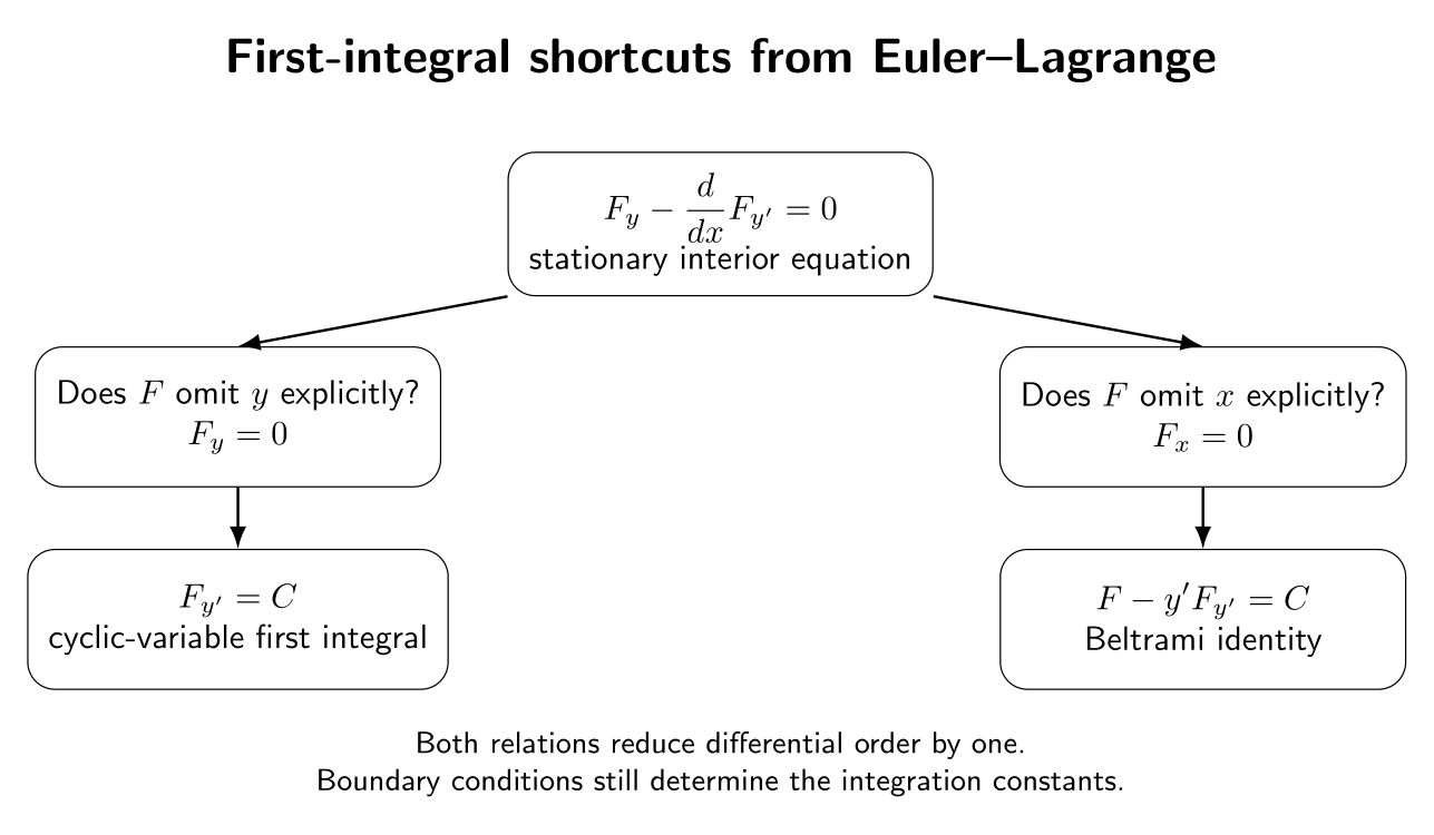
Figure. Two special structures produce immediate first integrals. If the dependent variable
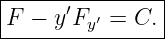
y is absent explicitly, the conjugate quantity Fy′ is constant. If the independent variable x
is absent explicitly, the Beltrami quantity F − y′Fy′ is constant.
1 Learning objectives
After completing CV06, the reader should be able to
- recognize when an Euler–Lagrange problem has a cyclic dependent variable;
- derive the first integral Fy′ = C when Fy = 0;
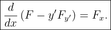
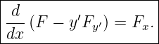
- derive the du Bois–Reymond identity
 (F − y′Fy′) = Fx along a stationary curve;
- obtain the Beltrami identity when Fx = 0;
- understand why a first integral reduces the differential order by one;
- use a first integral to convert a variational problem to a quadrature;
- connect the autonomous mechanical case to conservation of energy;
- distinguish the cases Fy = 0 and Fx = 0; and
- recognize these first integrals as elementary precursors of Noether’s theorem.
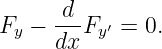
2 Starting point: the Euler–Lagrange equation
Consider the first-order functional
with F sufficiently smooth and with a stationary curve y∗(x) smooth enough for the derivatives
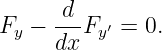
below to exist. CV04 derived the necessary interior condition
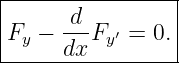
Throughout this article, the partial derivatives of F are evaluated along the candidate curve unless
stated otherwise.
A generic equation of this form contains y′′ through
If Fy′y′≠0, solving Euler–Lagrange therefore normally requires a second-order differential equation
and two boundary conditions. A first integral replaces that second-order equation by a first-order
relation.
3 First special form: the dependent variable is cyclic
Suppose the integrand has no explicit dependence on y:
Then
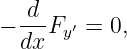
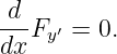
Euler–Lagrange immediately becomes
or
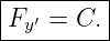
Therefore
The variable y is called a cyclic or ignorable variable because it does not appear explicitly in F.
The derivative
is often called the momentum conjugate to y. In an abstract variational problem this is simply
useful terminology; in mechanics it becomes canonical momentum under the usual identification
F = L [4, 5].
3.1 Why “cyclic” does not mean constant
A common misconception is that if y is absent from F, then y itself must be constant. That is
false. The conserved quantity is
which may be a nonlinear function of y′ and may also depend explicitly on x.
For example, let
Then
The first integral gives
so
A single integration yields
The stationary curve need not be constant even though y is cyclic.
4 The du Bois–Reymond identity
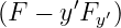
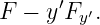
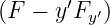
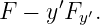
A second important reduction begins with the combination
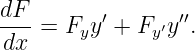
Differentiate it along an arbitrary sufficiently smooth curve:
Because
the total derivative of F is
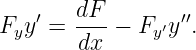
Substituting gives
  | = Fx + Fyy′ + Fy′y′′− y′′Fy′− y′ Fy′ Fy′ | (20)
|
| = Fx + y′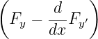 . . | (21) |
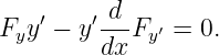
The two terms containing y′′Fy′ cancel identically. Along a stationary curve, Euler–Lagrange
makes the expression in parentheses vanish. Therefore
This relation is commonly called the du Bois–Reymond condition or du Bois–Reymond identity in
the classical theory [1, 2]. It is not an additional independent equation when the classical
Euler–Lagrange equation already holds with sufficient smoothness; rather, it is a useful
consequence of it.
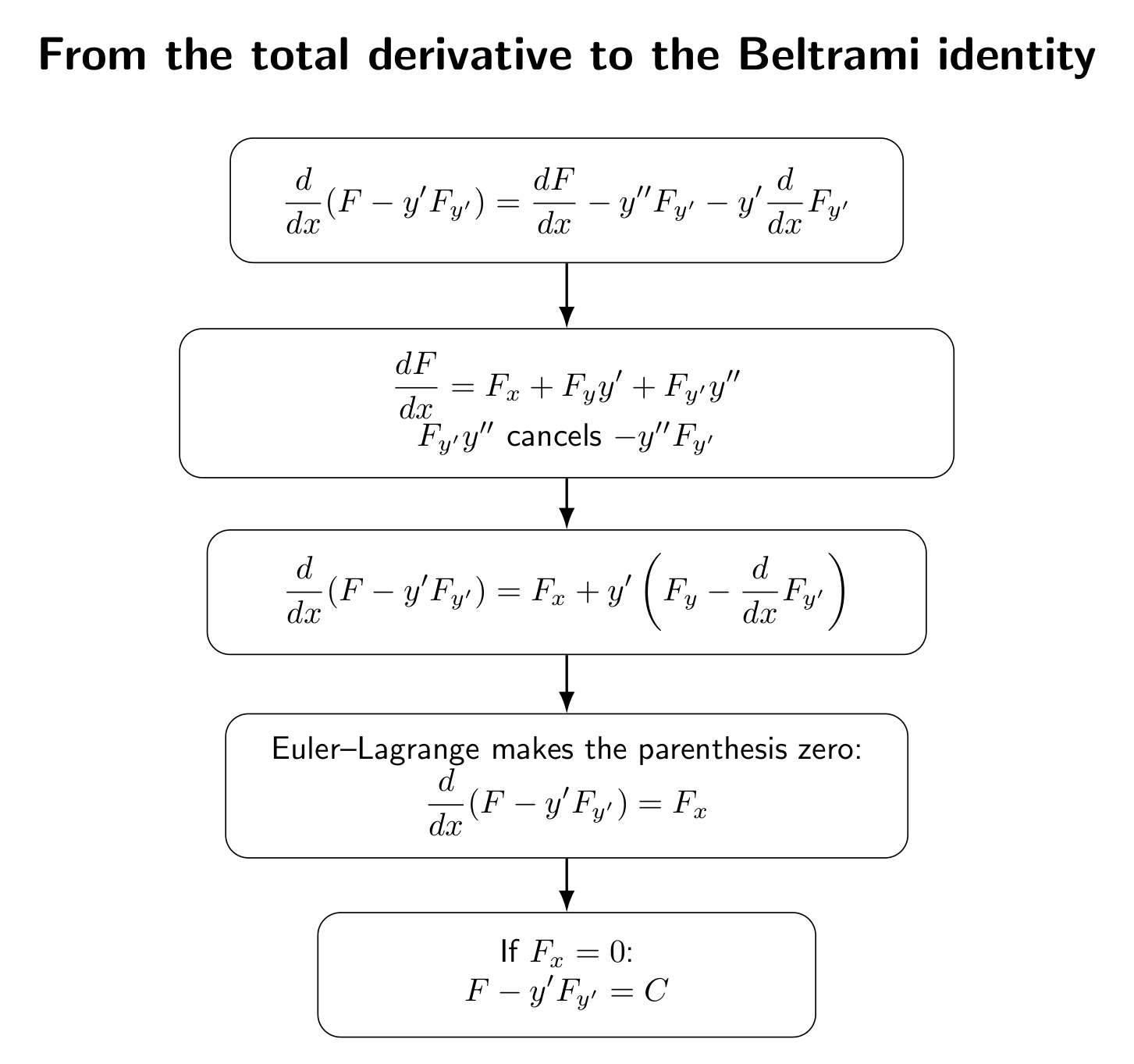
Figure. The derivative of F −y′Fy′ contains two cancellations. The chain-rule terms Fy′y′′
and −y′′Fy′ cancel algebraically; the remaining Euler–Lagrange residual vanishes on a
stationary curve.
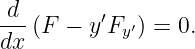
5 The Beltrami identity
Now suppose the integrand has no explicit dependence on the independent variable:
Then
The du Bois–Reymond identity reduces to
Hence
This is the Beltrami identity. It is one of the most useful first integrals in elementary calculus of
variations.
Some books write the same result with the opposite sign:
The two forms are equivalent because C1 = −C. What matters is the constancy, not the sign
convention.
6 Why a first integral is valuable
Euler–Lagrange is normally second order. A first integral has the schematic form
If this relation can be solved for y′, then
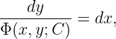
This is a first-order differential equation. In favorable cases it can be separated:
or rearranged into another directly integrable form. Thus the first integral has reduced the
differential order by one.
A first integral does not guarantee that the remaining first-order equation has an elementary
closed-form solution. It may only reduce the problem to a quadrature. That reduction is still
substantial.
7 Worked example 1: planar arc length revisited
Consider
The integrand is
It contains neither y nor x explicitly, so both special structures are available.
7.1 Using the cyclic-variable form
Since Fy = 0,
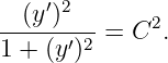
Square both sides:
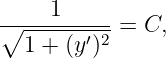
Therefore
so
As long as |C| < 1,
Hence
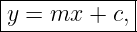
which is a straight line.
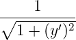
7.2 Using Beltrami instead
Because Fx = 0,
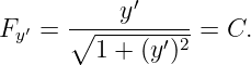
Substitute the arc-length integrand:
| F − y′Fy′ | = 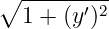 − −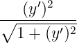 | (40)
|
| =  . . | (41) |
Therefore
which again implies constant slope.
The two first integrals are not independent in this simple example; both encode the same
straight-line geometry.
8 Worked example 2: a cyclic variable with explicit x dependence
Return to
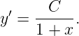
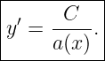
where a(x) > 0 is known. Because Fy = 0,
Thus
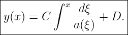
Integrating,
The constants C and D are then selected by the endpoint conditions.
Notice the distinction:
gives a first integral even though
Therefore the Beltrami identity does not apply, but the cyclic-variable integral does.
9 Worked example 3: autonomous mechanics and energy
In analytical mechanics the independent variable is time t and the dependent variable
is a generalized coordinate q(t). To keep the notation explicit, define the generalized
velocity
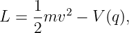
The integrand is the Lagrangian
If the Lagrangian has no explicit time dependence,
Beltrami gives
Define canonical momentum
Then
The quantity
is the Hamiltonian associated with the Lagrangian. Hence an autonomous Lagrangian
gives
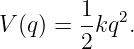
For the standard one-degree-of-freedom mechanical Lagrangian
we have
and therefore
| H | = v(mv) −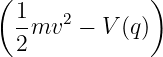 | (59)
|
| =  mv2 + V (q). mv2 + V (q). | (60) |
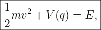
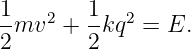
Thus
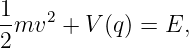
which is conservation of mechanical energy for this class of systems [4, 5].
9.1 Order reduction by the energy integral
From
we obtain
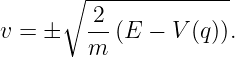
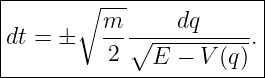
Therefore
The second-order equation of motion has been reduced to a first-order equation, and then to a
quadrature.
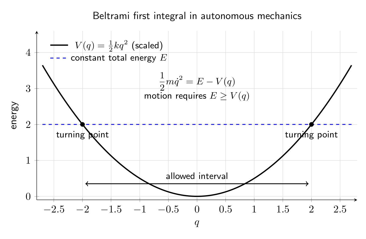
Figure. For an autonomous one-degree-of-freedom mechanical system, the Beltrami first
integral becomes conservation of energy. Motion is possible only where E ≥ V (q); the
intersections E = V (q) are turning points where v = 0.
10 Example 4: harmonic oscillator from the first integral
Let
Energy conservation gives
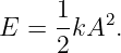
Suppose the turning-point amplitude is A. At q = A,
so
Substitution gives
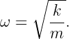
Define
Then
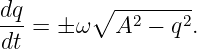
Since v = dq∕dt,
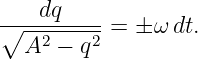
Separate variables:
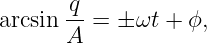
Integrating,
which yields the familiar sinusoidal motion
The first integral did not merely confirm energy conservation; it solved the motion by one
quadrature.
11 Worked example 5: a refractive-index invariant
A useful preview of variational optics is the functional
where the refractive index depends on height y but not explicitly on x. The integrand
is
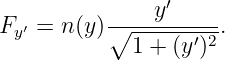
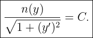
Because Fx = 0, Beltrami gives
Now
Hence
| F − y′Fy′ | = n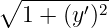 − n − n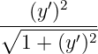 | (80)
|
| = 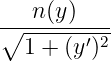 . . | (81) |
Therefore
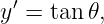
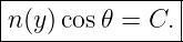
Let 𝜃 be the angle between the ray tangent and the positive x axis. Then
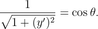
so
Thus
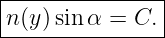
If instead the ray angle α is measured from the vertical normal to the horizontal index layers, then
α =  − 𝜃 and
This is the continuous-medium form of the same invariant underlying Snell’s law. CV16 will derive
Fermat’s principle and optical ray equations in full.
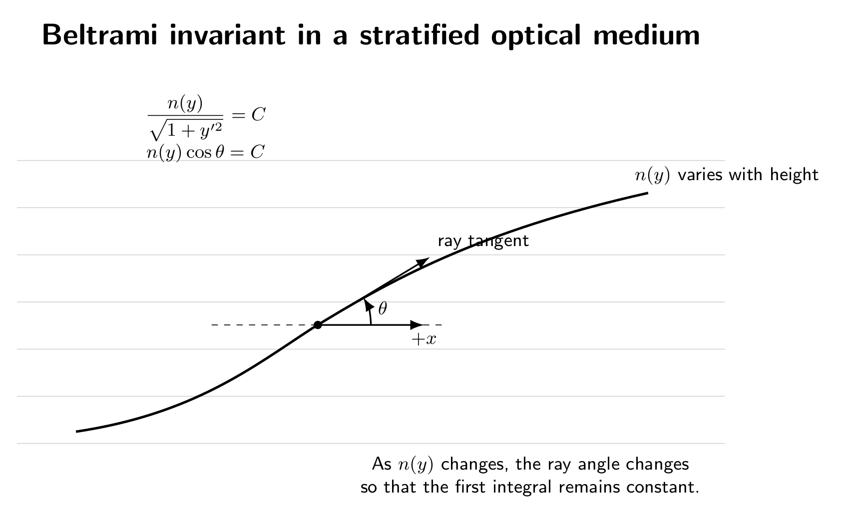
Figure. When the optical integrand is independent of x, the Beltrami invariant is constant
along the ray. The tangent angle changes as n(y) changes so that n cos 𝜃 remains fixed.
12 Do not confuse the two special cases
The two common first integrals come from different missing variables:
|
|
|
Structure | Euler–Lagrange
consequence | First integral |
|
|
|
Fy = 0 |  Fy′ = 0 Fy′ = 0
| Fy′ = C |
|
|
|
Fx = 0 |  (F − y′Fy′) = 0 (F − y′Fy′) = 0
| F − y′Fy′ = C |
|
|
|
both Fy = 0 and Fx =
0 | both reductions are
available | the resulting constants may be
algebraically related |
|
|
|
It is therefore useful to inspect the integrand before differentiating anything. A ten-second
structural check can save a page of second-order ODE algebra.
13 A compact derivation from Euler–Lagrange by multiplication
There is another way to see the Beltrami identity. Start from
Multiply by y′:
If Fx = 0, the total derivative of F is
Therefore
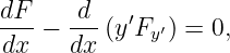
Substitute into the multiplied Euler–Lagrange equation:
But by the product rule,
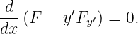
Hence
so
This derivation is algebraically equivalent to the du Bois–Reymond route but can be useful when
first learning the identity.
14 Endpoint conditions still matter
A first integral reduces the interior differential equation; it does not remove the boundary data
developed in CV05.
For example, suppose
and therefore
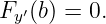
If the terminal value y(b) is free at a fixed b, CV05 gives the natural condition
Since Fy′ is constant along the entire extremal, this forces
The endpoint condition can therefore determine the first-integral constant immediately.
This is a recurring pattern:
15 First integrals and symmetry: a preview of Noether
The two reductions in this article already contain the seed of Noether’s theorem.
If Fy = 0, shifting the dependent variable by a constant,
does not change the integrand. The associated conserved quantity is
If Fx = 0, translating the independent variable,
does not change the explicit form of the integrand. The associated first integral is
In mechanics these become, respectively, momentum-like and energy-like conservation laws. CV20
will replace these special observations by the general Noether theorem for continuous
transformations.
16 Regularity and limitations
The derivations above use classical differentiability. A clean sufficient setting is
Then the chain rules and total derivatives used in the proofs are ordinary classical derivatives.
Several cautions are important.
- A first integral is a necessary consequence of stationarity under the stated hypotheses.
It does not by itself prove a minimum.
- If Fy′y′ = 0, the Euler–Lagrange equation can be degenerate, and the usual
interpretation as a second-order equation may fail.
- Solving a first integral for y′ may require choosing branches. Boundary conditions and
continuity determine which branch is admissible.
- A first integral may reduce the problem only to an implicit quadrature. An elementary
closed form is not guaranteed.
- If a stationary curve has corners, additional matching conditions are needed; these are
developed in CV10.
17 Common mistakes
- Mistake: using Beltrami whenever Fy = 0. Beltrami requires Fx = 0; the
cyclic-variable integral requires Fy = 0.
- Mistake: concluding that a cyclic variable is constant. The conserved object is Fy′,
not generally y.
- Mistake: dropping the sign difference between F − y′Fy′ and y′Fy′ − F. Both are
valid, but the integration constant changes sign.
- Mistake: calling y′Fy′ − F “energy” in every variational problem. It is a
Hamiltonian-like quantity; it becomes physical energy only under the appropriate
mechanical interpretation.
- Mistake: thinking a conserved quantity proves minimality. Conservation follows from
stationarity and symmetry, not from a second-variation test.
- Mistake: forgetting endpoint conditions after finding a first integral. The boundary
data still determine the constants and may eliminate entire branches of solutions.
18 A practical first-integral checklist
Given
use the following order of attack:
- Inspect which variables appear explicitly in F.
- If Fy = 0, write immediately
- If Fx = 0, write immediately
- If neither simplification applies, use the full Euler–Lagrange equation.
- Solve the first-order relation for y′ when possible.
- Integrate once more or reduce to a quadrature.
- Apply fixed, natural, or transversality boundary conditions from CV05.
- Keep the result labeled as a stationary candidate until a minimum or maximum classification
has been established separately.
19 Summary
For
Euler–Lagrange gives
If y is cyclic,
For any sufficiently smooth Euler–Lagrange extremal,
If x is absent explicitly, this becomes the Beltrami identity
These identities reduce the order of many variational differential equations and expose
conservation structures long before the general Noether theorem is available. CV06E1
will practice the Beltrami identity on several nonlinear problems, including classical
catenary-type reductions, while CV06E2 will focus on cyclic variables and conservation
laws. CV07 next extends Euler–Lagrange to several dependent variables and coupled
systems.
References
[1] I. M. Gelfand and S. V. Fomin, Calculus of Variations, Dover Publications, 2000.
[2] Bruce van Brunt, The Calculus of Variations, Springer, 2004.
[3] Robert Weinstock, Calculus of Variations with Applications to Physics and
Engineering, Dover Publications, 1974.
[4] Cornelius Lanczos, The Variational Principles of Mechanics, 4th ed., Dover
Publications, 1986.
[5] Herbert Goldstein, Charles Poole, and John Safko, Classical Mechanics, 3rd ed.,
Addison Wesley, 2002.

![∫
b ′
J[y] = F (x,y,y )dx,
a](https://images.physicslibrary.org/cache/objects/1202/make4ht/CalculusOfVariationsFirstIntegralsAndSpecialFormsOfTheEulerLagrangeEquation1x.png)



















![∫
b∘ ------′2-
J [y] = 1 + (y ) dx.
a](https://images.physicslibrary.org/cache/objects/1202/make4ht/CalculusOfVariationsFirstIntegralsAndSpecialFormsOfTheEulerLagrangeEquation36x.png)





![∫
b1 ′2
J[y] = 2-a(x)(y) dx,
a](https://images.physicslibrary.org/cache/objects/1202/make4ht/CalculusOfVariationsFirstIntegralsAndSpecialFormsOfTheEulerLagrangeEquation49x.png)















![∫
∘ ------′2-
J[y] = n (y ) 1 + (y) dx,](https://images.physicslibrary.org/cache/objects/1202/make4ht/CalculusOfVariationsFirstIntegralsAndSpecialFormsOfTheEulerLagrangeEquation82x.png)












![∫ b
J[y] = F (x,y,y′)dx,
a](https://images.physicslibrary.org/cache/objects/1202/make4ht/CalculusOfVariationsFirstIntegralsAndSpecialFormsOfTheEulerLagrangeEquation115x.png)


![∫ b
J[y] = F (x,y,y′)dx,
a](https://images.physicslibrary.org/cache/objects/1202/make4ht/CalculusOfVariationsFirstIntegralsAndSpecialFormsOfTheEulerLagrangeEquation118x.png)