Common Forces in Mechanics
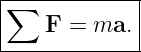
Newton’s second law does not determine the forces by itself. It tells how the net force changes
motion:
for a constant-mass particle. To use this equation, the physical interactions acting on the chosen
body must first be identified and modeled.
This article is a map of the force laws that occur most often in introductory mechanics. Each force
has three questions attached to it:
- What physical interaction produces the force?
- In what direction does the force act?
- What model determines its magnitude?
The answers are not interchangeable. A normal force, for example, is recognized from a surface
contact and points perpendicular to that surface, but its magnitude is usually found from Newton’s
second law rather than from a universal formula.
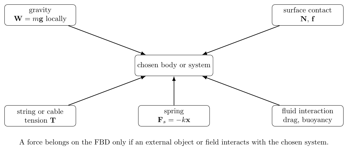
Figure 1. Common force models arise from identifiable interactions between the chosen system
and its environment. The force belongs on the free-body diagram only when that interaction
crosses the system boundary.
1 Force laws are models
A force law is a mathematical model for an interaction. Some are fundamental or long-range, such
as Newtonian gravity. Others are effective macroscopic descriptions of many microscopic
interactions, such as a normal force, friction, drag, or an elastic spring force.
The same object may experience several forces at once. The procedure is therefore
A label such as “applied force” describes how an external agent acts on the body, but it is not a
universal force law with one fixed magnitude formula.
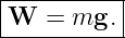
2 Weight
Near Earth’s surface, when The Gravitational Field can be treated as uniform, the gravitational
force on a body of mass m is
Its magnitude is
and its direction is vertically downward toward Earth.
The mass m is an intrinsic property of the object in Newtonian mechanics, while weight is a force
and therefore depends on the local gravitational field. A body can have the same mass in different
locations but different weights.
For problems extending over large distances, the uniform-field approximation may fail and
Newton’s inverse-square gravitational law must be used instead.
3 Normal force
When two surfaces press against one another, the contact interaction generally has a
component perpendicular to the surface. This perpendicular component is called the normal
force.
Its direction is fixed geometrically:
The normal force acts perpendicular to the contact surface and pushes the bodies
apart.
Its magnitude is not generally
That equality occurs only in particular situations. The correct value of N normally follows from
the force equation in the direction normal to the contact.
For example, if a block on a horizontal floor has no vertical acceleration and no other vertical
forces, then
so N = mg. If a rope pulls upward at an angle, or the supporting surface accelerates, the result
changes.
4 Friction
Friction is the component of a contact force tangent to the interface. Its direction opposes the
actual or impending relative sliding of the surfaces.
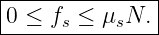
For static contact, the simple Coulomb model is
The static friction force adjusts to the value required by the dynamics, up to the limiting
magnitude
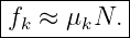
For surfaces sliding relative to one another, the introductory kinetic-friction model is
The kinetic-friction vector points opposite the relative sliding direction at the contact.
The coefficients μs and μk are empirical parameters. The simple Coulomb model is useful but not
universal.

Figure 2. Surface forces are resolved into a normal component perpendicular to the contact and a
friction component tangent to it. Their magnitudes must be determined from the appropriate
contact model and the equations of motion.
5 Tension
A taut string, rope, or cable pulls on the body attached to it. The force is directed along the string,
away from the body being analyzed.
For an ideal massless string passing over an ideal massless frictionless pulley, the Tension
magnitude is the same throughout one continuous string:
This equality is a model assumption, not a universal property of every rope or pulley system. A
massive rope can have different tension at different points because portions of the rope themselves
require net force to accelerate.
6 Spring force
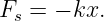
For an ideal linear spring, Hooke’s law is
where x is the displacement of the spring endpoint from its equilibrium position along the spring
axis and k is the spring constant.
In one dimension,
The minus sign expresses the restoring nature of the force: an extension produces a force toward
shorter length, while a compression produces a force toward longer length.
Hooke’s law is a linear approximation valid over the elastic range of the spring.
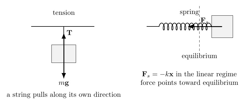
Figure 3. Tension acts along a taut string and pulls away from the body. An ideal linear spring
exerts a restoring force along the spring axis toward its equilibrium configuration.
7 Drag
A body moving relative to a fluid experiences a resistive force called drag. The important velocity
is the velocity relative to the fluid,
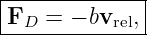
A common low-speed linear model is
where b is a positive drag coefficient.
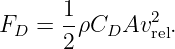
A common quadratic model is
with c > 0. In aerodynamic notation, the magnitude is often written
The direction of drag is opposite the relative velocity through the fluid. The correct drag model
depends on the flow regime, body geometry, and Reynolds number.
8 Buoyant force
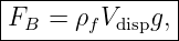
A body immersed in a fluid experiences a net pressure force that, in a hydrostatic fluid, gives the
buoyant force
where ρf is the fluid density and V disp is the displaced fluid volume.
The buoyant force points opposite the local effective direction of gravity; in the usual terrestrial
setting it points upward.
Although buoyancy belongs mainly to fluid mechanics, it is useful to recognize it as another
common external force in particle Free-body diagrams.
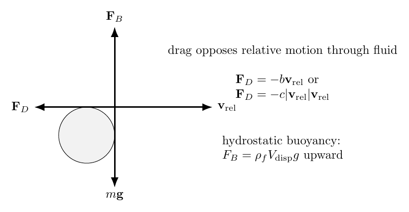
Figure 4. A fluid can exert both drag, which opposes relative motion through the fluid, and
buoyancy, which results from the pressure field in the fluid.
9 Applied and contact forces
Introductory problems often specify an “applied force” directly, such as a person pushing a crate
with 40 N. In that case the magnitude is given by the problem rather than by a separate
constitutive law.
Likewise, the contact force between two bodies may be left as an unknown vector or separated into
normal and tangential components. Newton’s third law then gives the corresponding force on the
other body:
These two forces act on different bodies and therefore should not both appear on one body’s
free-body diagram.
10 A compact force-recognition table
| Interaction | Typical direction | Introductory magnitude model |
|
|
|
| Gravity near Earth | downward | mg |
| Surface normal | perpendicular to surface | solve from dynamics |
| Static friction | tangent to surface | 0 ≤ fs ≤ μsN |
| Kinetic friction | opposite sliding | fk ≈ μkN |
| Tension | along taut string | solve from dynamics |
| Linear spring | toward equilibrium | Fs = k|x| |
| Linear drag | opposite vrel | FD = bvrel |
| Quadratic drag | opposite vrel | FD = cvrel2 |
| Buoyancy | upward in static fluid | ρfV dispg |
The table is a recognition aid, not a substitute for a free-body diagram. The direction and
magnitude assumptions must still match the physical situation.
11 Worked example 1: angled pull on a rough floor
A 10.0 kg crate is pulled by a rope with tension 50.0 N at 30.0∘ above the horizontal. The
kinetic-friction coefficient is μk = 0.20. Find the normal force, kinetic friction, and horizontal
acceleration. Use g = 9.81 m/s2.
The vertical force equation is
so
Numerically,
The kinetic friction is
Horizontally,
so
This example shows why N = mg should not be assumed: the upward component of tension
reduces the contact force.
12 Worked example 2: spring force and acceleration
A 4.0 kg block is attached to a horizontal spring with spring constant
The surface is frictionless. The block is displaced 0.080 m to the right of equilibrium. Find the
spring force and instantaneous acceleration.
Taking right as positive,
Hooke’s law gives
Thus
The negative signs indicate that both the spring force and acceleration point toward
equilibrium.
13 Worked example 3: falling body with quadratic drag
A 2.0 kg body falls downward through still air at 20.0 m/s. Model the drag magnitude
as
with
Find the instantaneous acceleration and the terminal speed predicted by this model.
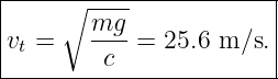
The drag acts upward because the velocity relative to the air is downward. Its magnitude
is
The weight magnitude is
Taking downward as positive,
so
downward.
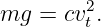
At terminal speed the net force is zero:
Therefore
14 Practice problems
- A 6.0 kg book rests on a horizontal table. Identify the forces on the book and determine
the normal force.
- A 3.0 kg lamp hangs motionless from one vertical ideal cord. Find the cord tension.
- A spring with k = 180 N/m is stretched 0.050 m from equilibrium. Find the spring-force
magnitude and state its direction.
- A 12 kg crate is pushed horizontally with 30 N and remains at rest. If μs = 0.40,
determine the actual static friction and verify that static equilibrium is possible.
- A 5.0 kg block slides on a horizontal surface with μk = 0.25. A horizontal force of 25
N pulls it to the right. Find the kinetic friction and acceleration.
- A small body moves east at 8.0 m/s through a fluid that itself moves east at 3.0 m/s.
If the linear drag law is FD = −bvrel with b = 2.0 kg/s, find the drag force.
- A fully submerged object displaces 0.0030 m3 of water of density 1000 kg/m3. Find the
buoyant-force magnitude using g = 9.81 m/s2.
- A block on a horizontal surface is pulled by a rope angled upward. Explain qualitatively
how increasing the upward component of the rope force changes the normal force and
therefore the maximum static friction μsN.
15 Answer check
- Weight 58.9 N downward and normal force 58.9 N upward.
- T = mg = 29.4 N.
- Fs = kx = 9.0 N toward equilibrium.
- The actual static friction is 30 N opposite the push. Since μsN = (0.40)(12)(9.81) =
47.1 N, static equilibrium is possible.
- fk = μkmg = 12.3 N; a = (25 − 12.3)∕5.0 = 2.55 m/s2 to the right.
- vrel = 5.0 m/s east, so the drag is 10.0 N west.
- FB = ρV g = (1000)(0.0030)(9.81) = 29.4 N upward.
- The upward rope component reduces N, so it also reduces the limiting static-friction
magnitude μsN.
16 Where the force models go next
This article is intentionally a hub. The following M02 articles develop the force models in more
detail:
- M02-04: weight, normal force, apparent weight, and curved support motion;
- M02-05: tension and massless strings;
- M02-06: pulleys and Atwood machines;
- M02-07: static and kinetic friction;
- M02-08: inclined-plane dynamics;
- M02-09: spring force and Hooke’s law;
- M02-10: drag and terminal velocity;
- M02-11: dynamics of circular motion.
17 Summary
The most useful force-modeling habit is to identify the interaction before writing a formula. Near
Earth’s surface, weight is modeled as mg; a surface can provide normal force and friction; a taut
string can provide tension; a spring can provide a restoring force; and a fluid can provide drag and
buoyancy. Once the individual forces have been modeled, Newton’s second law combines
them:
References
[1] PhysicsLibrary, M02-01, Newton’s Laws of Motion.
[2] PhysicsLibrary, M02-02, Free-Body Diagrams.
[3] J. Moore et al., Mechanics Map, force and particle-dynamics materials, CC BY-SA
4.0.
[4] University of California, Davis, Physics 9A Classical Mechanics materials, CC BY-SA
4.0.
[5] S. J. Ling, J. Sanny, and W. Moebs, University Physics, Volume 1, archived 2016 CC
BY 4.0 revision.