Line Integral in Physics: Curves, Work, Circulation, and Path Dependence
A line integral accumulates a quantity along a curve. In physics, line integrals appear
whenever a distributed quantity must be summed along a wire, trajectory, streamline, orbit,
or field line, or whenever a vector field does work along a path. They are central to
mechanics, gravitation, Electromagnetism, fluid mechanics, and Differential Geometry
[1, 2, 3, 4].
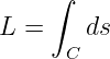
Two closely related but distinct forms occur repeatedly:
for a scalar field f, and
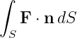
for a vector field F. The first weights each element of arc length by a scalar. The second measures
the component of a vector field along the directed tangent to the path.
The distinction between the scalar length element ds and the vector displacement element dr is
fundamental.
1 A curve as a vector-valued function
Let a curve C in three-dimensional space be parameterized by a scalar u:
For a regular smooth curve,
throughout the interval, except possibly at isolated junctions for a piecewise smooth
curve.
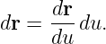
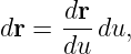
An infinitesimal displacement along the curve is
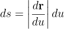
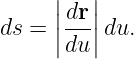
Its magnitude is the infinitesimal arc length,
Therefore
for an orientation in which u increases along the curve.
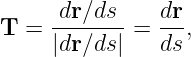
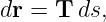
If T is the unit tangent,
then
Thus ds carries length only, while dr carries both length and direction.
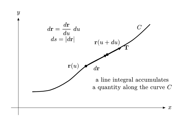
Figure 1. A parameterized curve and its differential displacement. The scalar element ds is the
magnitude of the directed vector element dr.
2 Scalar line integrals
Let f(r) be a scalar field defined along C. The scalar line integral is
Using the parameterization r(u),
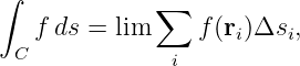
This formula is the precise meaning of “adding f along the curve.” A Riemann-sum interpretation
is
where the curve is divided into short segments of lengths Δsi.
2.1 Arc length as the simplest line integral
Set
Then
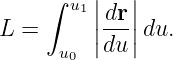
is simply the length of the curve. In parameter form,
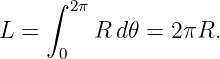
For a circle of radius R,
with 0 ≤ 𝜃 ≤ 2π. Since
we recover
2.2 Mass of a thin curved wire
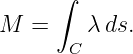
If a thin wire follows C and has linear mass density λ(r) with units kg/m, then
The dimensions make the interpretation transparent:
The same structure appears for Electric Charge distributed along a filament and for other scalar
densities defined per unit length.
3 Vector line integrals
Let F(r) be a vector field. The directed line integral of F along C is
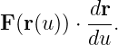
Using
we obtain
Since
we may also write
Only the tangent component of the field contributes.
4 Mechanical work as a line integral
The infinitesimal work done by a force through displacement dr is
If 𝜃 is the angle between F and the path tangent,
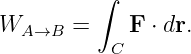
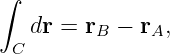
Therefore the total work from point A to point B along path C is
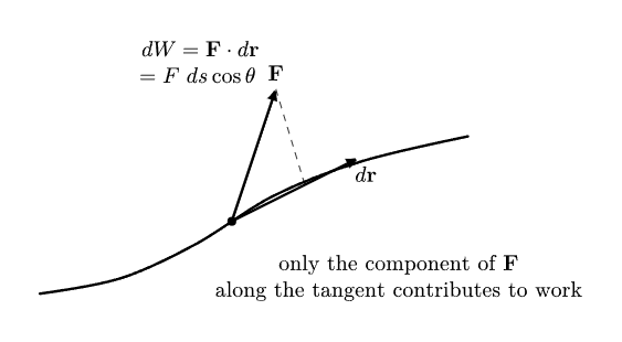
Figure 2. Work is the line integral of the component of force tangent to the path. A force
perpendicular to the instantaneous displacement does no infinitesimal work.
This definition contains several familiar facts. If the force is everywhere perpendicular to the
motion, then
and the force does no work. The magnetic part of the Lorentz force is a standard example
because
is perpendicular to v.
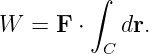
If F is constant,
But
so
For a constant force, only the endpoint displacement matters.
5 Orientation matters
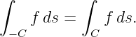
A scalar line integral with ds does not change if the path orientation is reversed, because ds is a
nonnegative length element:
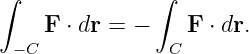
A vector line integral does change sign because dr reverses direction:
This orientation dependence is essential in work, circulation, and electromotive-force
calculations.
6 Independence of parameterization
A geometric line integral should depend on the curve, not on how quickly the parameter moves
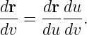
along it. Suppose the same oriented curve is described by
where g is differentiable and increases monotonically. Then
Substitution into the parameterized form shows that the factor du∕dv is exactly compensated by
the change of integration variable. Thus the line integral is invariant under any smooth
orientation-preserving reparameterization.
If the new parameter reverses orientation, the scalar ds integral remains unchanged while the
directed dr integral changes sign.
7 Path dependence
For a general vector field, the value of
can depend on the entire path between the endpoints.
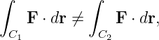
Let C1 and C2 connect the same points A and B. If
then the field is path dependent in that region.
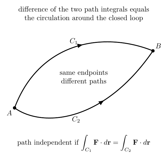
Figure 3. Two curves connect the same endpoints. A vector line integral is path independent only
when every admissible path between the endpoints gives the same value.
The difference between the two directed path integrals is a closed-loop integral. Traverse C1 from
A to B and return along −C2:
Therefore path independence is equivalent to vanishing circulation around every closed loop in the
region.
8 Conservative fields and potentials
A vector field is conservative in a region if there exists a scalar potential function Φ such
that
In mechanics it is more common to define potential energy V by
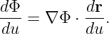
Let a curve be parameterized by u. By the chain rule,
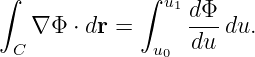
Therefore
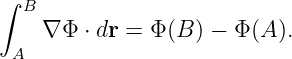
Hence
This is the fundamental theorem for line integrals.
For a conservative mechanical force,
Thus
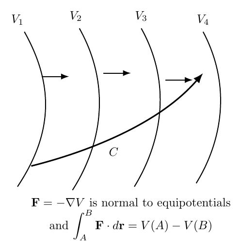
Figure 4. For a conservative force F = −∇V , the force is normal to surfaces of constant potential
and the work depends only on the endpoint values of V .
9 Example: work done by uniform gravity
Near Earth’s surface, let
For any path from height yA to height yB,
Then
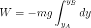
Therefore
and
The horizontal shape of the path does not matter. This is exactly the path independence expected
from the potential energy
10 Closed line integrals and circulation
A line integral around a closed curve is commonly written
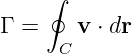
In fluid mechanics, if F is the fluid velocity v, then
is the circulation around the loop.
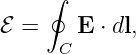
In electromagnetism, closely related line integrals occur in Maxwell’s Equations. Examples include
electromotive force,
and Ampere-Maxwell circulation,
The notation dl is often used instead of dr when emphasizing a directed line element along a
contour.
11 Connection with curl and Stokes’ theorem
For a sufficiently smooth vector field and an oriented surface S whose boundary is C, Stokes’
theorem states
Thus circulation around the boundary is related to curl distributed across the enclosed
surface.
If
throughout a simply connected region, then every closed-loop line integral vanishes there and F is
conservative.
The phrase “simply connected” matters. A region with a hole can support a curl-free field whose
circulation around a loop enclosing the hole is nonzero. A standard two-dimensional example away
from the origin is
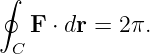
The curl vanishes wherever (x,y)≠(0, 0), but around a circle centered on the excluded
origin,
So “curl zero” and “path independent” are equivalent only when the topology and regularity
assumptions are satisfied.
12 Line integrals in generalized coordinates
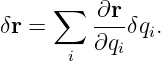
Suppose a particle position depends on generalized coordinates qi:
For an allowed virtual displacement at fixed time,
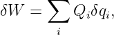
The virtual work is
Therefore
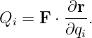
where the generalized force is
This is a direct extension of the same tangent-projection idea underlying the ordinary work line
integral.
13 A differential-form viewpoint
The expression
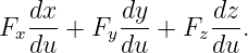
can be written in Cartesian coordinates as
Mathematically, this is a differential one-form integrated along a curve. The curve parameterization
pulls that one-form back to an ordinary one-variable integral:
This viewpoint becomes valuable in advanced mechanics, electromagnetism, differential geometry,
and relativity because it separates the geometric object being integrated from the coordinates used
to describe it.
14 What a line integral is not
Several related integrals should not be confused.
A time integral such as
is an integral over time. It may describe a path through configuration space, but its measure is dt,
not spatial arc length ds.
A surface integral such as
accumulates flux through a two-dimensional surface rather than along a one-dimensional
curve.
A volume integral accumulates throughout a three-dimensional region. The dimension
of the domain and the differential element determine what kind of integral is being
performed.
15 A practical calculation procedure
For a line integral in physics, the following sequence is reliable:
- Identify the geometric path C and its orientation.
- Choose a convenient parameter u and write r(u).
- Compute dr∕du.
- For a scalar line integral, compute
- For a vector line integral, substitute the path into F and compute
- Integrate over the parameter interval.
- Check dimensions, orientation, and whether a potential-function shortcut is available.
16 Summary
A line integral is an integral whose domain is a curve. Its two most common forms in physics
are
and
The scalar element ds measures distance along the curve, while the vector element dr carries the
tangent direction. Mechanical work is the vector line integral of force, circulation is a closed vector
line integral, and conservative-force work reduces to a difference of potential energies.
Parameterization is a computational device; the geometric integral itself depends on the oriented
curve. Stokes’ theorem then connects closed line integrals to curl and forms a bridge from
mechanics into electromagnetism and field theory.
References
References
[1] J. R. Taylor, Classical Mechanics, University Science Books, 2005.
[2] J. B. Marion and S. T. Thornton, Classical Dynamics of Particles and Systems, 5th
ed., Brooks/Cole, 2004.
[3] D. J. Griffiths, Introduction to Electrodynamics, 4th ed., Cambridge University Press,
2017.
[4] H. M. Schey, Div, Grad, Curl, and All That: An Informal Text on Vector Calculus,
4th ed., W. W. Norton, 2005.
[5] G. B. Arfken, H. J. Weber, and F. E. Harris, Mathematical Methods for Physicists,
7th ed., Academic Press, 2013.