Celestial Mechanics: Initial-Value Orbital Motion - Worked Problems and Complete
Solutions
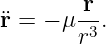
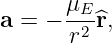
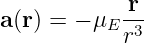
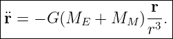
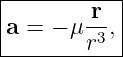
CM03 converted Newton’s gravitational force law into the point-mass orbital equation
The equation determines acceleration from position, but it does not by itself select a unique
trajectory. An orbital initial-value problem also requires
This companion article develops that idea through complete worked examples. It begins with direct
evaluation of gravitational acceleration, then treats circular motion and minimum-energy escape as
special initial conditions. It next works a fully three-dimensional Cartesian state, decomposes
velocity into radial and transverse parts, constructs a short-time state estimate, treats the exact
Earth–Moon two-body relative equation, and closes with a numerical Runge–Kutta propagation
experiment.
The goal is not yet to derive orbital elements. Instead, the emphasis is the physics of the
differential equation: given position and velocity now, what can we say immediately about
acceleration, energy class, and subsequent motion? [1, 2, 3, 4, 5].
Unless otherwise stated, use
For Earth–Moon examples use
and
Part I: Exercises
Exercise 1: acceleration from a Cartesian position
A spacecraft is at
relative to Earth’s center.
- Compute the distance r0 from Earth’s center.
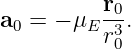
- Use Newton’s orbital equation to compute the acceleration vector a0.
- Find its magnitude.
- Explain why the acceleration is not small even though the spacecraft is in low Earth
orbit.
Exercise 2: circular orbit as a special initial condition
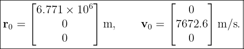
A spacecraft is at altitude
above Earth’s mean surface. At t0 let
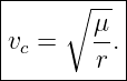
- Derive the speed required for a circular orbit by equating Newtonian gravitational
acceleration to centripetal acceleration.
- Evaluate the circular speed numerically.
- Compute the orbital acceleration magnitude.
- Derive and evaluate the circular period.
- Write the complete six-component initial state.
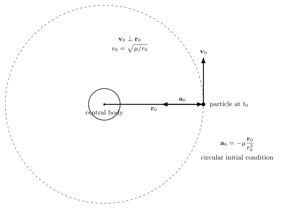
Figure. A circular initial condition has v0 ⊥ r0 with exactly the speed required for gravity
to provide the inward centripetal acceleration.
Exercise 3: minimum-energy radial escape trajectory
At the same 400 km altitude, launch a particle directly radially outward. Neglect atmosphere and
all bodies except Earth.
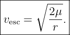
- Starting from conservation of specific mechanical energy, derive the minimum escape
speed at radius r0.
- Evaluate the escape speed numerically.
- Write a Cartesian initial state for a radial outward escape beginning on the +x axis.
- Compute the initial gravitational acceleration vector.
- Explain what happens to the speed as r →∞ at the exact escape threshold.
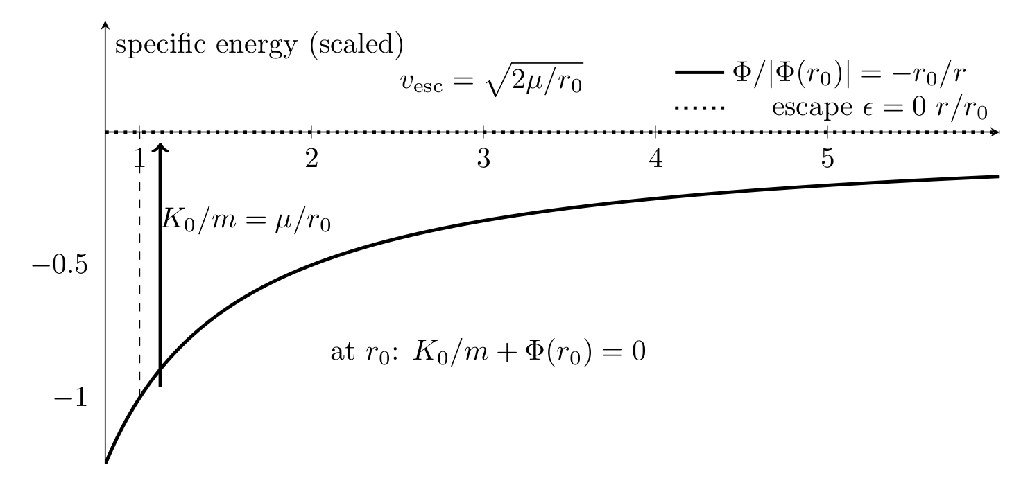
Figure. Minimum escape corresponds to zero total specific mechanical energy: the positive
launch kinetic energy exactly cancels the negative gravitational potential at the initial
radius.
Exercise 4: a sub-escape radial launch and turnaround radius
A particle is launched radially outward from Earth’s mean surface at
- Compute its initial specific mechanical energy.
- Determine whether it escapes.
- At the maximum radius the radial speed is zero. Use energy conservation to derive the
turnaround radius rmax.
- Compute the maximum altitude above Earth’s mean surface.
Exercise 5: a super-escape launch and hyperbolic excess speed
A particle is launched radially outward from Earth’s mean surface at
- Compute the initial specific mechanical energy.
- Show that the motion is unbound.
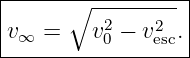
- Derive the speed v∞ remaining as r →∞.
- Evaluate v∞ numerically.
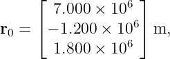
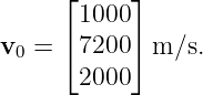
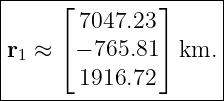
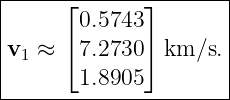
Exercise 6: a fully general Cartesian initial state
Consider the Earth-centered state
- Compute r0 = |r0| and v0 = |v0|.
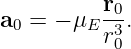
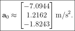
- Compute the gravitational acceleration vector.
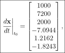
- Write the six-state derivative
 t0.
t0.
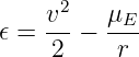
- Compute the specific mechanical energy 𝜖 and determine whether the state is
energetically bound or unbound.
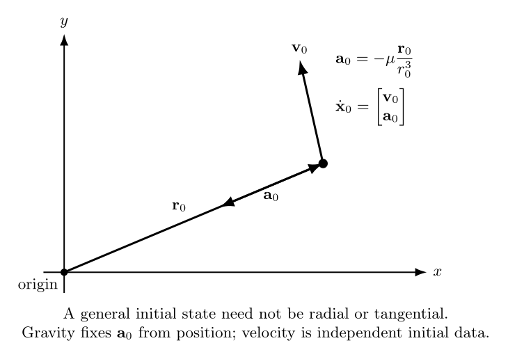
Figure. In a general Cartesian state, the velocity need not be radial or tangential.
Newton’s equation determines acceleration solely from the instantaneous position.
Exercise 7: radial and transverse velocity components
Use the Cartesian state from Exercise 6.
- Construct the radial unit vector r0.
- Compute the radial velocity
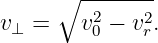
- Compute the magnitude of the velocity perpendicular to r0 from
- Is the spacecraft instantaneously moving inward or outward?
- Explain why the gravitational acceleration has no transverse component in the
radial-transverse decomposition.
Exercise 8: short-time propagation from the initial state
Again use the state from Exercise 6 and a short interval
Assume the acceleration remains approximately equal to a0 over this short interval.
- Use
to estimate the new position.
- Use
to estimate the new velocity.
- Explain why repeatedly using one fixed acceleration would eventually become
inaccurate.
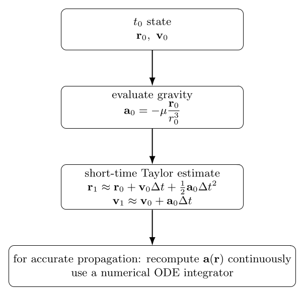
Figure. A short-time Taylor step uses the acceleration evaluated at the initial position.
Accurate orbit propagation requires continuously updating the acceleration as the position
changes.
Exercise 9: energy classification for several initial speeds
At 400 km altitude, suppose the velocity is perpendicular to the radius. For each speed below,
compute
and classify the state as negative-energy bound, zero-energy escape threshold, or positive-energy
unbound:
- v = 7.00 km/s;
- v = vcirc;
- v = 9.00 km/s;
- v = vesc;
- v = 12.0 km/s.
Explain why energy classification alone does not tell us the complete geometric shape or
orientation of the orbit.
Exercise 10: changing velocity without changing instantaneous gravity
Two spacecraft occupy exactly the same position
but have different velocities:
- Compute the instantaneous acceleration of each spacecraft.
- Are the accelerations equal?
- Are the future trajectories the same?
- What does this demonstrate about the role of initial velocity in a second-order orbital
differential equation?
Exercise 11: exact Earth–Moon relative acceleration
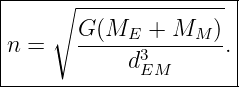
Treat Earth and Moon as two point masses separated by dEM.
- Compute the Moon’s acceleration toward Earth from Earth’s gravity alone.
- Compute Earth’s acceleration toward the Moon.
- Add the magnitudes appropriately to obtain the relative acceleration magnitude.
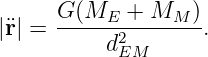
- Verify the exact relative-motion formula
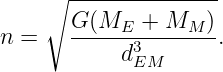
- Explain why using only GME is an approximation to the exact relative problem.
Exercise 12: barycentric circular initial conditions for Earth and Moon
Assume, for this exercise, a perfectly circular Earth–Moon two-body orbit of fixed separation
dEM.
- Compute the distances rE and rM of Earth and Moon from their common center of
mass.
- Derive the common angular speed
- Compute the corresponding Earth and Moon barycentric speeds.
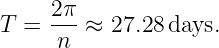
- Compute the orbital period of this idealized circular two-body system.
- Write one set of barycentric Cartesian initial position and velocity vectors that gives
counterclockwise circular motion in the xy plane.
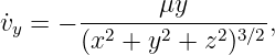
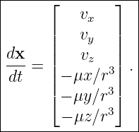
Exercise 13: write the orbital equation as a six-state first-order system
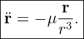
Define
- Write all six scalar first-order differential equations equivalent to
- Identify which state components determine the instantaneous gravitational acceleration.
- Explain why this form is convenient for numerical ODE solvers.
Exercise 14: Julia RK4 propagation of a circular initial state
Use the 400 km circular initial state from Exercise 2.
- Write a Julia function that computes dx∕dt from the six-state vector.
- Implement one classical fourth-order Runge–Kutta step.
- Propagate exactly one theoretical circular period using N = 1000 equal steps.
- Compare the final numerical position and velocity with the initial values.
- Compute the specific mechanical energy before and after propagation and use the
difference as one numerical quality check.
Part II: Complete Worked Solutions
Solution 1: acceleration from a Cartesian position
The given position is already along the positive x axis:
Therefore
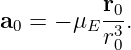
Newton’s orbital equation is
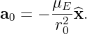
Because the position lies along +x,
Numerically,
 | = 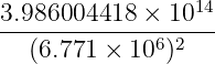 | (31)
|
| ≈ 8.6943 m/s2. | (32) |
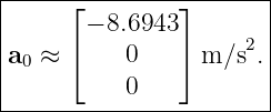
Thus
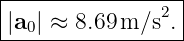
Its magnitude is
This is only modestly smaller than surface gravity. Low Earth orbit is therefore not a region in
which gravity has disappeared. Orbital motion is continuous free fall under a still-strong
gravitational acceleration.
Solution 2: circular orbit as a special initial condition
The orbital radius is
| r0 | = RE + h | (35)
|
| = 6.371 × 10⁶ + 4.00 × 10⁵ | (36)
|
| = 6.771 × 10⁶ m. | (37) |
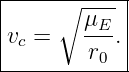
For uniform circular motion, the required centripetal acceleration is
Gravity supplies that acceleration:
Multiply by r0:
Therefore
Numerically,
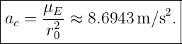
The acceleration magnitude is
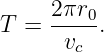
The circumference is 2πr0, so the period is
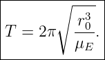
Substituting vc =  gives
gives
Numerically,
One convenient initial state is
The velocity is perpendicular to the radius, and its magnitude is exactly the value required for
circular motion.
Solution 3: minimum-energy radial escape trajectory
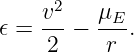
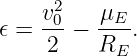
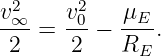
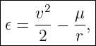
The specific mechanical energy is
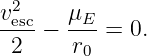
For minimum escape, the particle reaches infinity with zero remaining speed. Therefore
Energy conservation requires
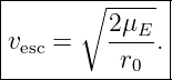
Hence
At 400 km altitude,
For a radial outward launch from the positive x axis, one suitable initial state is
The initial acceleration is still determined only by position:
The velocity points outward while gravity points inward, so the particle slows continuously. At the
exact escape threshold,
The particle never reaches a finite turnaround radius; it asymptotically approaches zero speed at
infinite distance.
Solution 4: a sub-escape radial launch and turnaround radius
At Earth’s surface,
and
The specific energy is
| 𝜖 | =  − − | (58)
|
| ≈−2.2065 × 10⁷ J/kg. | (59) |
Thus
so the launch does not escape.
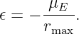
At the maximum radius, the radial speed is zero. Therefore
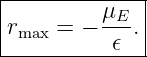
Solve for rmax:
Numerically,
Therefore the maximum altitude is
| hmax | = rmax − RE | (64)
|
| ≈ 11694 km. | (65) |
Thus
This is a useful reminder that a very large launch speed can still correspond to a bound trajectory
if it remains below local escape speed.
Solution 5: a super-escape launch and hyperbolic excess speed
At the surface,
With v0 = 12.0 km/s,
Thus the motion is unbound.
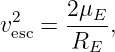
At infinity, gravitational potential tends to zero, so
Equating the initial and final energies gives
Using
we obtain
With
we find
This residual speed is often called the hyperbolic excess speed in astrodynamics.
Solution 6: a fully general Cartesian initial state
Convert the state to SI units:
The radius magnitude is
| r0 | =  | (77)
|
| ≈ 7.32666 × 10⁶ m. | (78) |
Thus
The speed is
| v0 | =  | (80)
|
| ≈ 7539.23 m/s. | (81) |
Therefore
Now evaluate
The result is approximately
The six-state derivative is therefore
where the first three entries have units of m/s and the final three have units of m/s2.
The specific mechanical energy is
| 𝜖 | =  − − | (86)
|
| ≈−2.5984 × 10⁷ J/kg. | (87) |
Thus
so the ideal two-body trajectory is energetically bound.
Solution 7: radial and transverse velocity components
The radial unit vector is
Using the values from Exercise 6,
The radial speed is
| vr | = v0 ⋅r0 | (91)
|
| ≈ 267.5 m/s. | (92) |
Thus
The positive sign means that the spacecraft is instantaneously moving outward.
The perpendicular speed is
| v⊥ | =  | (94)
|
| ≈ 7534.5 m/s. | (95) |
Hence
The gravitational acceleration is
so it is purely radial. Its transverse component is exactly zero for an ideal central point-mass
gravity field.
Solution 8: short-time propagation from the initial state
Use
and the acceleration from Exercise 6.
The second-order position estimate is
Evaluating component by component gives approximately
The first-order velocity estimate is
which gives
The new position magnitude is about
The approximation eventually fails if we keep the same a0 because gravitational acceleration
changes in both magnitude and direction as r changes. Numerical orbit propagation therefore
repeatedly evaluates
at updated positions.
Solution 9: energy classification for several initial speeds
At 400 km altitude,
and
For v = 7.00 km/s,
so the state is bound.
For the circular speed vc ≈ 7.6726 km/s,
This is also
for a circular orbit.
For v = 9.00 km/s,
so the state is still bound.
For v = vesc ≈ 10.8507 km/s,
which is the escape threshold.
For v = 12.0 km/s,
so the state is unbound.
The sign of energy classifies bound versus threshold versus unbound motion, but it does not
determine the full orbit. The direction of v and the angular momentum are also required to
determine orbital geometry and orientation.
Solution 10: changing velocity without changing instantaneous gravity
Both spacecraft have exactly the same position:
The point-mass acceleration depends only on position:
Therefore both spacecraft have
Numerically,
Their accelerations are equal at that instant, but their future trajectories are not the same
because their initial velocities differ. A second-order differential equation needs both
position and velocity initial conditions. Position fixes the instantaneous gravitational
acceleration; velocity determines how the state begins moving through the acceleration
field.
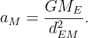
Solution 11: exact Earth–Moon relative acceleration
The Moon’s acceleration toward Earth is
Numerically,
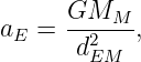
Earth’s acceleration toward the Moon is
so
The accelerations point toward one another. For the relative coordinate
its second derivative is the difference of the individual acceleration vectors. Because the vectors are
opposite in the inertial frame, the relative acceleration magnitude is the sum of the two
magnitudes:
| |r| | = aM + aE | (122)
|
| ≈ 2.7308 × 10⁻³ m/s2. | (123) |
Directly,
which verifies
Using only GME neglects Earth’s motion and is therefore a test-particle approximation. It is often
useful because MM ≪ ME, but it is not the exact two-body relative equation.
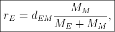
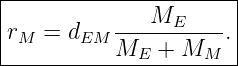
Solution 12: barycentric circular initial conditions for Earth and Moon
Let the center of mass be the origin. The two distances from the barycenter satisfy
and
Therefore
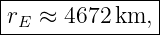
Numerically,
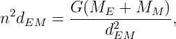
For circular relative motion,
so
Numerically,
The barycentric speeds are
and
The period is
One counterclockwise set of barycentric initial conditions is
These choices keep the center of mass at rest and make both bodies rotate counterclockwise about
it.
Solution 13: write the orbital equation as a six-state first-order system
Let
The kinematic equations are
The acceleration components are
and
Thus
Only the position components x,y,z determine the instantaneous point-mass gravitational
acceleration. The velocity components are still essential because they determine the complete state
and therefore which trajectory is followed through the field.
Most general-purpose numerical ODE integrators are designed for systems of first-order equations.
Writing orbital dynamics in six-state form therefore allows the same standard algorithms used for
many other dynamical systems to propagate an orbit.
Solution 14: Julia RK4 propagation of a circular initial state
A compact Julia implementation is:
using LinearAlgebra
using Printf

const muE = 3.986004418e14
const RE  = 6.371e6
const h   = 400e3
const r0mag = RE + h
const vc = sqrt(muE / r0mag)
const T  = 2pi * sqrt(r0mag^3 / muE)

function rhs(x)
    r = x[1:3]
    v = x[4:6]
    rn = norm(r)
    a = -muE .* r ./ rn^3
    return vcat(v, a)
end

function rk4_step(x, dt)
    k1 = rhs(x)
    k2 = rhs(x .+ (0.5 * dt) .* k1)
    k3 = rhs(x .+ (0.5 * dt) .* k2)
    k4 = rhs(x .+ dt .* k3)
    return x .+ (dt/6.0) .* (k1 .+ 2 .* k2 .+ 2 .* k3 .+ k4)
end

function specific_energy(x)
    r = x[1:3]
    v = x[4:6]
    return dot(v,v)/2 - muE/norm(r)
end

x0 = [r0mag, 0.0, 0.0, 0.0, vc, 0.0]
x = copy(x0)

N = 1000
dt = T / N
E0 = specific_energy(x0)


for k in 1:N
    x = rk4_step(x, dt)
end

Ef = specific_energy(x)

dr = norm(x[1:3] - x0[1:3])
dv = norm(x[4:6] - x0[4:6])

@printf("period = %.6f s\n", T)
@printf("dt = %.6f s\n", dt)
@printf("position closure error = %.6e m\n", dr)
@printf("velocity closure error = %.6e m/s\n", dv)
@printf("specific-energy change = %.6e J/kg\n", Ef-E0)
The theoretical circular period is
With N = 1000,
A representative RK4 run gives a position closure error on the order of
and a velocity closure error on the order of
The specific-energy change is approximately
for this step size and one-orbit propagation.
The exact numbers depend on floating-point arithmetic and implementation details, but the
important check is that the propagated state closes closely after one theoretical period and that
the conserved energy changes only slightly. Later numerical celestial-mechanics lessons will
compare general-purpose Runge–Kutta methods with symplectic integrators designed for long-term
hamiltonian motion.
1 What CM03E1 adds to the series
CM03 established the initial-value problem
CM03E1 shows how to use it in practice.
For circular motion,
For minimum escape,
For a completely general Cartesian state, the acceleration is still simply
while the velocity supplies independent initial data that selects the actual trajectory.
The problem set also introduced the useful energy classifier
without yet deriving the full conic orbit. The next theory lessons can now expose the deeper
conservation structure hidden in Newton’s equation, beginning with angular momentum and
planar motion.
References
[1] J. M. A. Danby, Fundamentals of Celestial Mechanics, 2nd ed., Willmann-Bell, 1988.
[2] Roger R. Bate, Donald D. Mueller, and Jerry E. White, Fundamentals of
Astrodynamics, Dover Publications, 1971.
[3] John R. Taylor, Classical Mechanics, University Science Books, 2005.
[4] Herbert Goldstein, Charles P. Poole, and John L. Safko, Classical Mechanics, 3rd ed.,
Addison-Wesley, 2001.
[5] Bradley W. Carroll and Dale A. Ostlie, An Introduction to Modern Astrophysics, 2nd
ed., Pearson Addison-Wesley, 2007.

![[parent]](https://images.physicslibrary.org/images/uparrow.png)



















![x = [x y z v v v ]T .
x y z](https://images.physicslibrary.org/cache/objects/1276/make4ht/CelestialMechanicsInitialValueOrbitalMotionWorkedProblemsAndCompleteSolutions25x.png)