Celestial Mechanics: Gravitational Potential and Spherical Gravity - Worked Problems and
Complete Solutions
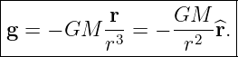
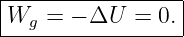
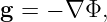
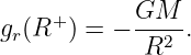
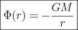
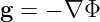
CM02 introduced gravitational work, potential energy, gravitational potential, and the
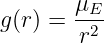
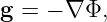
relation
This companion article develops those ideas through complete worked problems. The first problems
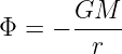
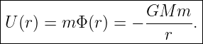
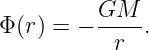
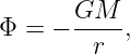
stay close to the point-mass potential
and its corresponding potential energy
The later problems extend the same reasoning to spherical shells and uniform solid spheres. The
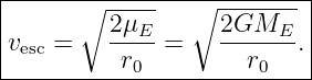
escape-speed derivation is included explicitly because it is the first major celestial-mechanics
application of gravitational potential energy.
Unless otherwise stated, use
and
Part I: Exercises
Exercise 1: gravitational work between two radii
A mass m moves radially outward from r1 to r2, where r2 > r1, in the field of a point mass
M.
- Starting from Fg = −GMmr∕r2, derive the gravitational work W
g(r1 → r2).
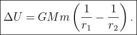
- Derive the corresponding change in potential energy ΔU.
- Explain the signs of Wg and ΔU for outward motion.
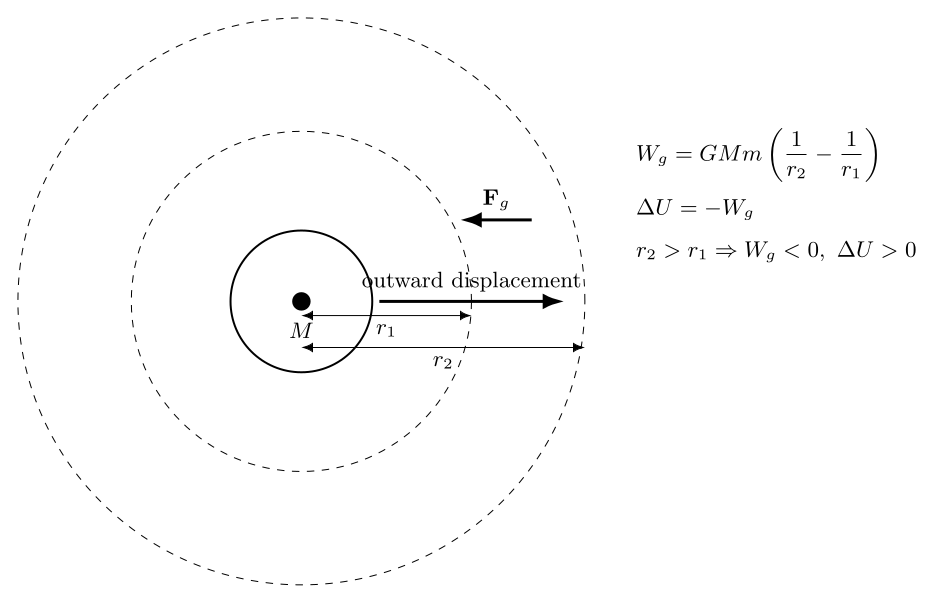
Figure. Outward motion is opposite the gravitational force. Gravity therefore does
negative work while the gravitational potential energy increases.
Exercise 2: Earth’s surface gravitational potential
Using the point-mass exterior approximation for Earth:
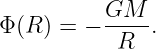
- calculate the gravitational potential Φ(RE) at Earth’s mean surface;
- calculate the potential energy of a 1000 kg spacecraft at that location;
- explain why both values are negative when the reference Φ(∞) = 0 is chosen.
Exercise 3: exact altitude energy change versus mgh
Raise a 1.00 kg mass from Earth’s mean surface to altitude
- calculate the exact change in gravitational potential energy using −μEm∕r;
- estimate the change using mg0h, where g0 = μE∕RE2;
- compute the percentage by which the constant-g approximation differs from the exact
result;
- explain the source of the difference.
Exercise 4: recover the gravitational field from the potential
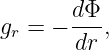
For a point mass,
Use
and spherical symmetry to recover the familiar point-mass gravitational field. Carefully track the
sign.
Exercise 5: work along an equipotential surface
A test mass moves along a circular arc of constant radius r around a spherical gravitating
body.
- What is the change in gravitational potential ΔΦ?
- What is the gravitational work Wg?
- Show the same result directly from Fg ⋅ dr.
- Explain why equipotential surfaces are perpendicular to The Gravitational Field.
Exercise 6: scalar superposition of gravitational potential
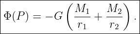
Two point masses M1 and M2 produce a gravitational potential at a point P.
- Write the total potential in terms of distances r1 and r2 from P.
- Evaluate the potential at the midpoint between Earth and Moon.
- Explain why potentials add as scalars even though gravitational fields add as vectors.
Exercise 7: zero gravitational field does not mean zero potential
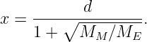
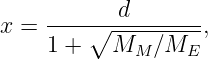
Use the Earth–Moon zero-field point derived in CM01E1,
where x is measured from Earth’s center toward the Moon.
- calculate x and the distance d − x from the Moon;
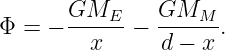
- calculate the gravitational potential there;
- explain how g = 0 can coexist with Φ≠0.
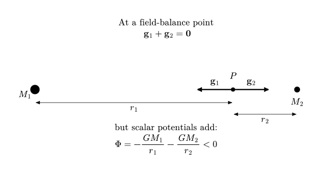
Figure. Vector gravitational fields can cancel at a point, while the scalar gravitational
potentials from positive masses remain additive and negative when zero is chosen at infinity.
Exercise 8: derive and calculate Earth’s escape speed
A mass m is launched from Earth’s mean surface with just enough speed to reach infinity with zero
remaining speed.
- Write the initial and final mechanical energies.
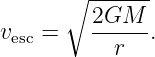
- Derive the escape-speed formula
- calculate Earth’s surface escape speed.
- explain why the escaping object’s mass cancels.
- explain why mgh is not the correct potential-energy model for escape to infinity.
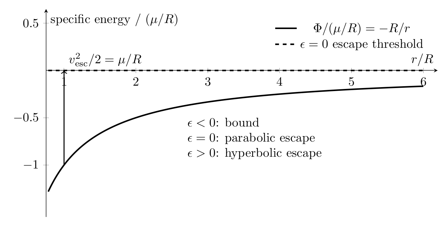
Figure. Escape threshold corresponds to zero total specific mechanical energy. Negative
specific energy is bound; zero is the parabolic threshold; positive is unbound.
Exercise 9: escape speed from low Earth orbit altitude
At altitude 400 km above Earth’s mean surface:
- calculate the local escape speed;
- compare it with the surface escape speed;
- calculate the circular-orbit speed at the same radius using vcirc =
 ;
;
- verify the relation vesc =
 vcirc.
Exercise 10: potential of a thin spherical shell
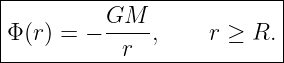
A thin spherical shell has total mass M and radius R. Use the shell theorem and the convention
Φ(∞) = 0.
- determine Φ(r) for r ≥ R;
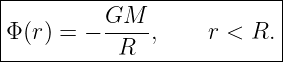
- determine Φ(r) for r < R;
- show that Φ is continuous at r = R;
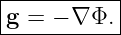
- use g = −∇Φ to recover the exterior and interior fields.
Exercise 11: field inside a uniform solid sphere
A solid sphere has radius R, total mass M, and constant density.
- find the enclosed mass M(r) for r < R;
- use the shell theorem to derive the field inside the sphere;
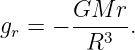
- show that the field magnitude grows linearly with r;
- verify that the interior field matches the exterior surface field at r = R.
Exercise 12: potential inside a uniform solid sphere
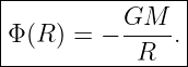
Using the field from Exercise 11 and continuity with the exterior potential at r = R, derive the
interior potential
Then find:
- the potential at the surface;
- the potential at the center;
- the potential difference between center and surface.
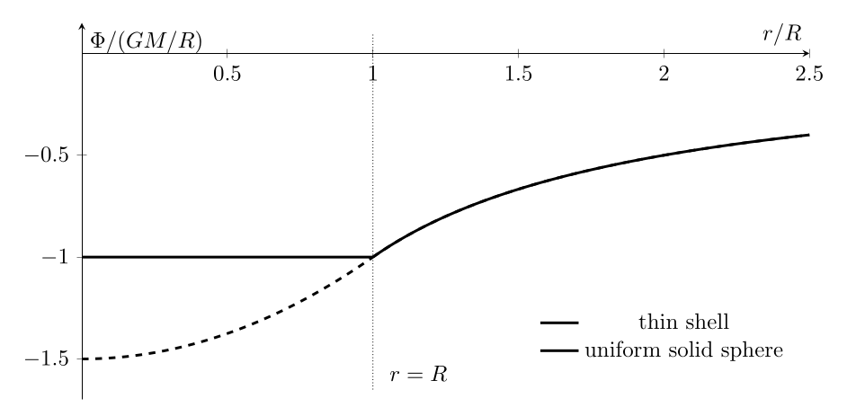
Figure. A thin shell has constant interior potential, while a uniform solid sphere has a
quadratic interior potential. Both match the exterior −GM∕r potential continuously at the
surface.
Exercise 13: escape speed from the center of a uniform sphere
Imagine a hypothetical nonrotating Earth with the same total mass ME and radius RE but
uniform density. Ignore tunnels, pressure, and material interactions.
- use the interior potential to derive the escape speed from the center;
- calculate its numerical value;
- compare it with the surface escape speed.
Exercise 14: continuity of potential and behavior of the field at a surface
Compare a thin spherical shell and a uniform solid sphere of equal M and R.
- show that Φ is continuous across r = R for both objects;
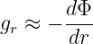
- determine whether the radial field gr = −dΦ∕dr is continuous across r = R for the
thin shell;
- determine whether it is continuous for the uniform solid sphere;
- explain physically why the answers differ.
Exercise 15: Julia check of spherical field and potential profiles
Write a Julia program that evaluates Φ(r) and gr(r) for
- a thin spherical shell;
- a uniform solid sphere;
using normalized units G = M = R = 1.
Check numerically that
away from the thin shell’s surface, and verify continuity of Φ at r = R for both models.
Part II: Complete Worked Solutions
Solution 1: gravitational work between two radii
For radial motion,
Therefore
| Wg | = ∫
r1r2
Fg ⋅ dr | (16)
|
| = −GMm∫
r1r2
r−2 dr | (17)
|
| = −GMm![[ 1]
− --
r](https://images.physicslibrary.org/cache/objects/1252/make4ht/CelestialMechanicsGravitationalPotentialAndSphericalGravityWorkedProblemsAndCompleteSolutions17x.png) r1r2 r1r2
| (18)
|
| = GMm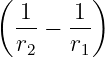 . . | (19) |
Thus
For a conservative force,
Hence
If r2 > r1, then 1∕r2 < 1∕r1, so
Gravity points inward while the displacement is outward, so gravity removes kinetic energy unless
some external agent supplies energy. The gravitational potential energy becomes less negative as
the body is moved farther away.
Solution 2: Earth’s surface gravitational potential
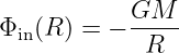
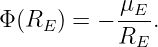
The potential is
Substituting the given values,
| Φ(RE) | = −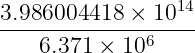 | (25)
|
| ≈−6.2565 × 10⁷ J/kg. | (26) |
Thus
For a 1000 kg spacecraft,
| U | = mΦ | (28)
|
| = (1000)(−6.2565 × 10⁷) | (29)
|
| ≈−6.2565 × 10¹⁰ J. | (30) |
Therefore
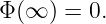
The negative sign follows from the convention
At any finite distance from an attractive positive mass, energy must be added to move a
test mass all the way to infinity. The finite-distance state therefore lies below the zero
reference.
Solution 3: exact altitude energy change versus mgh
The initial radius is
and the final radius is
For m = 1.00 kg,
| ΔU | = μEm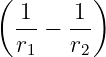 | (35)
|
| ≈ 3.6960 × 10⁶ J. | (36) |
So
The surface gravitational acceleration from the same spherical model is
| g0 | =  | (38)
|
| ≈ 9.8203 m/s2. | (39) |
The constant-g estimate is
| mg0h | = (1)(9.8203)(4.00 × 10⁵) | (40)
|
| ≈ 3.9281 × 10⁶ J. | (41) |
Thus
The relative difference is approximately
Hence the constant-g model overestimates the energy change by about
The reason is that mgh assumes the surface value of g acts over the entire height. In
reality,
decreases continuously as the mass rises.
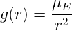
Solution 4: recover the gravitational field from the potential
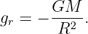
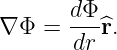
For spherical symmetry,
With
we have
Therefore
| g | = −∇Φ | (50)
|
| = − r. r. | (51) |
Thus
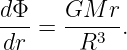
The derivative dΦ∕dr is positive because the negative potential rises toward zero as r increases.
The extra minus sign in g = −∇Φ makes the field point toward decreasing potential, which is
inward.
Solution 5: work along an equipotential surface
At constant radius r,
is constant. Therefore
For a test mass m,
Hence
We can see the same result directly. Along a circular arc, dr is tangent to the circle while gravity is
radial. Therefore
and
Thus gravity does no work along an equipotential surface. More generally, since
the field points normal to surfaces of constant Φ.
Solution 6: scalar superposition of gravitational potential
For point masses,
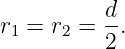
At the midpoint between Earth and Moon,
Therefore
| Φmid | = −G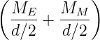 | (62)
|
| = −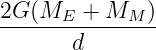 . . | (63) |
Numerically,
Potential is a scalar, so each source contributes one signed scalar value and the contributions are
added directly. The gravitational field is a vector, so its source contributions must be added with
direction.
Solution 7: zero gravitational field does not mean zero potential
The balance point satisfies
Using the stated masses and separation,
Its distance from the Moon is
| d − x | ≈ 3.8380 × 10⁷ m | (67)
|
| ≈ 38380 km. | (68) |
The potential is
Numerically,
At this location the two field vectors are equal in magnitude and opposite in direction,
so
But the potentials are both negative scalars:
They therefore add rather than cancel. A zero gradient does not imply a zero value of the scalar
function. It means only that the local slope vanishes.
Solution 8: derive and calculate Earth’s escape speed
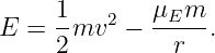
The total mechanical energy of a mass m in Earth’s field is
For minimum escape from radius r0, the object reaches infinity with speed approaching zero.
Therefore
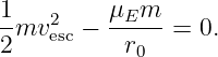
Energy conservation gives
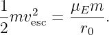
Thus
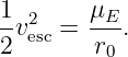
Cancel m:
Therefore
At Earth’s mean surface,
| vesc | = 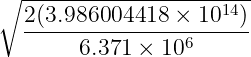 | (79)
|
| ≈ 1.1186 × 10⁴ m/s. | (80) |
Thus
The escaping object’s mass cancels because both kinetic energy and gravitational potential energy
are proportional to m.
The approximation mgh is not suitable for escape to infinity because it assumes nearly constant
gravitational acceleration. Escape traverses distances comparable with and much larger than
Earth’s radius, over which
changes drastically. The exact −μEm∕r potential must be used.
Solution 9: escape speed from low Earth orbit altitude
The radius at 400 km altitude is
The local escape speed is
| vesc | =  | (84)
|
| ≈ 1.0851 × 10⁴ m/s. | (85) |
Therefore
This is smaller than the surface value 11.19 km/s because some gravitational potential energy has
already been gained by climbing to the higher radius.
The circular speed at the same radius is
| vcirc | =  | (87)
|
| ≈ 7.6726 km/s. | (88) |
Then
 vcirc vcirc | ≈ 1.4142(7.6726) | (89)
|
| ≈ 10.85 km/s, | (90) |
so
at the same radius in an inverse-square point-mass field.
Solution 10: potential of a thin spherical shell
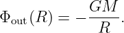
For r ≥ R, the shell theorem says the gravitational field is the same as that of a point mass M at
the center. With zero potential at infinity,
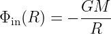
At the surface,
Inside a thin spherical shell, the shell theorem gives
Since
zero field means the potential is spatially constant throughout the interior. Continuity with the
surface fixes that constant:
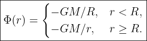
Thus the complete potential is
The potential is continuous at r = R.
Taking the radial derivative gives
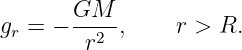
and
The field jumps at the idealized surface because the mass density is concentrated in an
infinitesimally thin layer.
Solution 11: field inside a uniform solid sphere
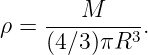
The constant density is
At radius r < R, the enclosed mass is
| M(r) | = ρ πr3 πr3 | (101)
|
| = M . . | (102) |
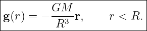
By the shell theorem, spherical shells outside radius r make no net contribution to the field at that
interior point. Therefore
| gr(r) | = − | (103)
|
| = − . . | (104) |
Thus
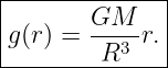
Its magnitude is
The field therefore grows linearly from zero at the center.
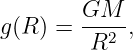
At r = R,
which matches the exterior point-mass field at the surface. Unlike the ideal thin shell, a uniform
volume density does not create a jump in g at the outer boundary.
Solution 12: potential inside a uniform solid sphere
For r < R,
Since
we have
Integrate from the surface R to an interior radius r:
Therefore
Φ(r) − | =  (r2 − R2). (r2 − R2). | (112) |
Rearranging,
| Φ(r) | = − + +  (r2 − R2) (r2 − R2) | (113)
|
| = − + +  . . | (114) |
Thus
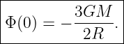
At the surface,
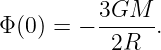
At the center,
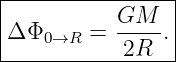
The potential difference from center to surface is
| Φ(R) − Φ(0) | = − + +  | (118)
|
| =  . . | (119) |
Hence
The potential rises smoothly from its most negative value at the center to the surface value, then
approaches zero as −GM∕r outside.
Solution 13: escape speed from the center of a uniform sphere
At the center of a uniform sphere,
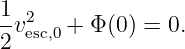
Minimum escape again corresponds to zero total specific mechanical energy at infinity:
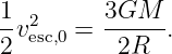
Thus
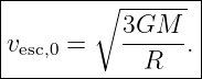
Therefore
For the hypothetical uniform Earth,
| vesc,0 | =  | (125)
|
| ≈ 1.3700 × 10⁴ m/s. | (126) |
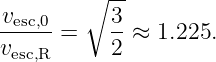
Hence
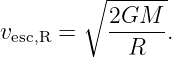
At the surface,
Thus
The center requires a greater escape speed because the potential is deeper even though the local
gravitational field is zero exactly at the center. Again, field strength and potential value are
distinct concepts.
Solution 14: continuity of potential and behavior of the field at a surface
For the thin shell,
and
So Φ is continuous.
Inside the shell,
Just outside,
Therefore the field has a jump discontinuity across the ideal infinitesimally thin mass
layer.
For the uniform solid sphere,
matches the exterior value, so the potential is again continuous.
The interior field approaches
while the exterior field approaches
Thus the field is also continuous for the uniform sphere.
The distinction comes from the mass distribution. A thin shell has finite surface mass density
concentrated on a zero-thickness layer, producing a jump in the normal gravitational field. A
uniform solid sphere has a finite volume density with no singular surface layer, so the field
transitions continuously.
Solution 15: Julia check of spherical field and potential profiles
One implementation is:
using Printf

G = 1.0
M = 1.0
R = 1.0

function phi_shell(r)
    r < R ? -G*M/R : -G*M/r
end

function g_shell(r)
    r < R ? 0.0 : -G*M/r^2
end

function phi_solid(r)
    if r <= R
        return -G*M/(2R) * (3 - r^2/R^2)
    else
        return -G*M/r
    end
end

function g_solid(r)
    if r <= R
        return -G*M*r/R^3
    else
        return -G*M/r^2
    end
end

function numerical_g(phi, r; dr=1e-5)
    return -(phi(r + dr) - phi(r - dr))/(2dr)
end

println(" r       shell g: a/n       solid g: a/n")
for r in (0.25, 0.75, 0.99, 1.01, 1.5, 2.0)
    @printf("%.2f   % .5f/% .5f   % .5f/% .5f\n",
            r, g_shell(r), numerical_g(phi_shell, r),


            g_solid(r), numerical_g(phi_solid, r))
end

println("\nPotential continuity check near r = R")
for r in (0.999999, 1.0, 1.000001)
    @printf("r=%.6f  shell Phi=% .9f  solid Phi=% .9f\n",
            r, phi_shell(r), phi_solid(r))
end
Away from r = R, the centered finite difference should satisfy
For the thin shell, the derivative is not defined at the idealized surface because the field jumps
there. The potential itself remains continuous.
For the uniform solid sphere, both Φ and its first radial derivative are continuous at r = R, so
the numerical derivative passes smoothly through the surface when the resolution is
adequate.
1 What CM02E1 adds to the series
CM02 introduced potential as an alternative description of Newtonian gravity. CM02E1 develops
the practical consequences:
The escape-speed derivation demonstrates why potential energy is so valuable in celestial
mechanics: a problem that would require integrating a continuously changing acceleration can
instead be solved from one scalar conservation equation.
The spherical examples also establish several ideas that recur throughout astrophysics:
- exterior spherical gravity behaves like a point mass;
- a field can vanish where the potential is nonzero;
- potential is usually smoother than the field;
- the interior potential depends on the mass distribution, not merely the total mass;
- escape is determined by the depth of the potential well.
The next main lesson can now return to dynamics and derive Newton’s orbital equation of motion
from the gravitational field.
References
[1] Bradley W. Carroll and Dale A. Ostlie, An Introduction to Modern Astrophysics, 2nd
ed., Pearson/Addison-Wesley, 2007.
[2] Herbert Goldstein, Charles Poole, and John Safko, Classical Mechanics, 3rd ed.,
Addison-Wesley, 2001.
[3] John R. Taylor, Classical Mechanics, University Science Books, 2005.
[4] J. M. A. Danby, Fundamentals of Celestial Mechanics, 2nd ed., Willmann-Bell, 1988.
[5] Roger R. Bate, Donald D. Mueller, and Jerry E. White, Fundamentals of
Astrodynamics, Dover Publications, 1971.

![[parent]](https://images.physicslibrary.org/images/uparrow.png)



















 (
(