Celestial Mechanics: Newton’s Law of Universal Gravitation
Celestial mechanics begins with a force law. Before discussing ellipses, orbital elements, Kepler’s
equation, perturbations, or three-body motion, we first need a precise mathematical statement of
how two masses attract one another.
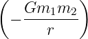
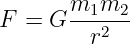
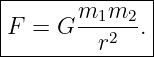
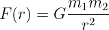
Newton’s law of universal gravitation says that two point masses m1 and m2, separated by distance
r, attract each other with force magnitude
This compact expression contains several distinct pieces of physics:
- the interaction is proportional to each mass;
- it becomes weaker with the square of separation;
- the force acts along the line joining the masses;
- the force is attractive;
- the two bodies exert equal and opposite forces on one another.
The purpose of CM01 is to unpack those statements carefully and express them in the vector
language needed for later celestial mechanics. The lesson also introduces The Gravitational Field,
superposition, continuous mass distributions, the gravitational parameter, and the first
astronomical-scale calculations. The potential formulation is previewed here and developed
systematically in CM02 [6, 2, 3, 1].
1 From a scalar force magnitude to a vector law
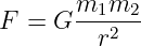
The scalar expression
tells us the size of the force but not its direction. Orbital motion requires a vector equation.
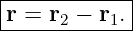
Let the inertial positions of the masses be
Define the relative displacement from body 1 to body 2 by
Its magnitude is
and the corresponding unit vector is
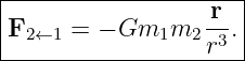
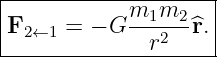
The force on body 2 due to body 1 must point from body 2 back toward body 1, opposite to r.
Therefore
Using
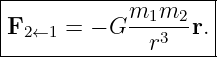
we obtain the form used throughout celestial mechanics:
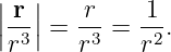
The factor r3 in the denominator sometimes looks surprising because the familiar scalar law
contains r2. There is no contradiction. The vector r contributes one factor of length:
2 Attraction and the minus sign
The minus sign is geometric, not decorative.
By definition,
points from body 1 toward body 2. Gravity on body 2 points the opposite way, toward body 1.
Therefore its direction is
If instead one defines the relative vector in the opposite direction, the algebraic sign in the force
law changes accordingly. What is physically invariant is that the gravitational force points toward
the attracting mass.
This is why defining the relative position vector explicitly is essential before writing a vector force
law.
3 Newton’s third law for the pair
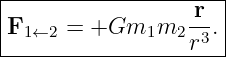
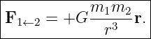
The force on body 1 due to body 2 points from body 1 toward body 2:
Thus
This is Newton’s third law for the isolated gravitational pair.
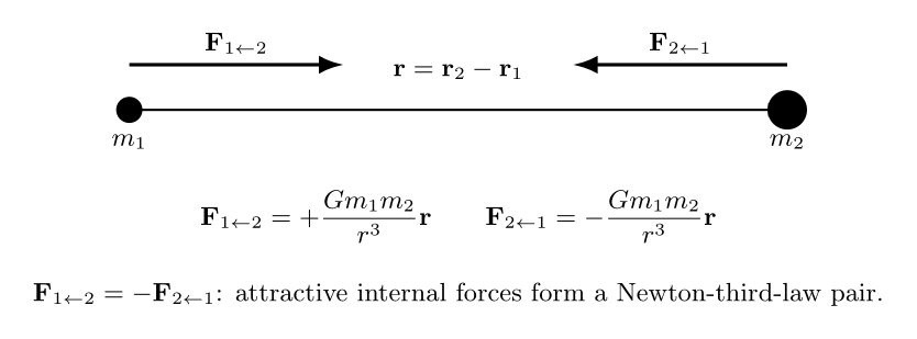
Figure. With r = r2 − r1, gravity pulls each body toward the other. The two internal
forces have equal magnitude and opposite direction.
The third-law structure becomes important in CM08, where the exact two-body problem is
separated into center-of-mass motion and relative motion.
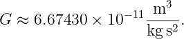
4 The gravitational constant G
The constant G sets the strength of Newtonian gravitation. In SI units,
Unlike the speed of light in SI, G is not fixed by definition; it is determined experimentally.
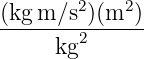
Its dimensions can be recovered from the force law. Since
we require
| [G] | = ![[F ][r]2
-------
[m ]2](https://images.physicslibrary.org/cache/objects/1249/make4ht/CelestialMechanicsNewtonsLawOfUniversalGravitation16x.png) | (17)
|
| =  | (18)
|
| =  . . | (19) |
This dimensional check is useful because celestial-mechanics formulas often contain the
combination GM, whose units are
That combination will soon become so common that it receives its own symbol.
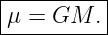
5 The gravitational parameter
For a dominant central mass M, define the gravitational parameter
Then the gravitational acceleration due to a point mass can be written compactly as
In the exact relative two-body problem, the corresponding parameter becomes
which will be derived later rather than assumed.
Using μ is often preferable in practical orbital work because planetary and stellar gravitational
parameters can be determined very accurately from dynamical observations.
6 Why an inverse-square dependence?
Newtonian gravity has the radial dependence
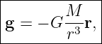
There is an important geometrical reason that inverse-square laws appear naturally in
three-dimensional space.
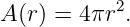
The area of a sphere of radius r is
If some conserved radial flux is distributed uniformly across spherical surfaces, then the flux per
unit area must scale as
At twice the radius,
so the same total flux is spread over four times the area.
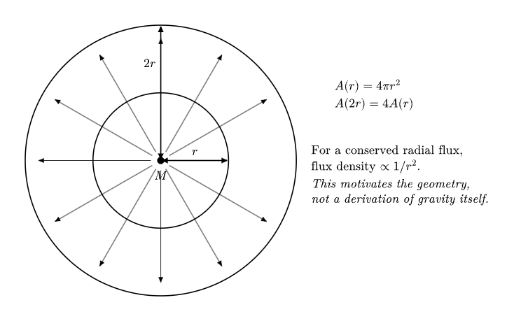
Figure. The area of a sphere grows as r2, so any conserved spherically symmetric radial
flux has a density proportional to 1∕r2. This explains the geometry associated with an
inverse-square field, but does not by itself derive Newton’s gravitational law.
That last distinction matters. Geometry explains why a conserved radial flux has inverse-square
behavior. It does not prove that gravity must be such a flux or determine the coupling strength G.
Newtonian gravitation is a physical law supported by observation; the spherical-area argument
helps us understand its spatial structure.
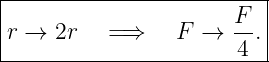
7 A simple scaling consequence
If the separation changes from r to 2r, the force changes from
to
| F(2r) | = G | (29)
|
| =  F(r). F(r). | (30) |
Thus
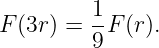
If the separation triples,
This rapid weakening with distance is central to nearly every approximation used later in celestial
mechanics.
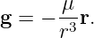
8 From force to gravitational field
It is often useful to separate the property of the source from the mass of the object used to probe
it.
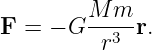
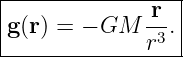
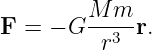
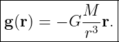
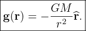
Suppose a source mass M is located at the origin and a test mass m is at position r. The
gravitational force on the test mass is
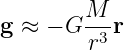
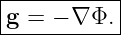
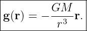
Define the gravitational field as force per unit test mass:
Therefore
Equivalently,
Its units are
Thus the gravitational field is also an acceleration field.
9 Why the test mass cancels
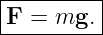
Newton’s second law gives
But gravitational force is
Therefore
For nonzero m,
In Newtonian gravity, the acceleration produced by a given external gravitational field is
independent of the test body’s mass.
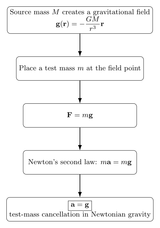
Figure. The source mass creates the gravitational field. Multiplying the field by a test
mass gives the force, and Newton’s second law then cancels that test mass, leaving a = g.
This cancellation is the Newtonian manifestation of the equivalence between inertial
and gravitational mass. General relativity later elevates this observation into a much
deeper geometrical principle, but Newtonian celestial mechanics only requires the result
a = g.
10 Example 1: gravitational acceleration at Earth’s surface
Treat Earth as spherically symmetric and use
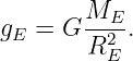
The Newtonian surface gravitational acceleration is
Substituting,
| gE | = (6.67430 × 10⁻¹¹)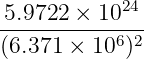 | (45)
|
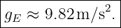
| ≈ 9.82 m/s2. | (46) |
Thus
The familiar near-surface value of g is therefore not a separate law. It is the local value of Earth’s
gravitational field.
Real measured surface gravity varies because Earth rotates, is oblate rather than perfectly
spherical, has altitude variations, and possesses nonuniform mass distribution. Those refinements
belong to gravitational-field modeling rather than the ideal point-mass law.
11 Example 2: the Sun’s gravitational acceleration at Earth
Let
and take one astronomical unit as
The Sun’s gravitational field magnitude at Earth’s orbital distance is
| g⊙(1 AU) | = G | (50)
|
| ≈ 5.93 × 10⁻³ m/s2. | (51) |
Therefore
This is much smaller than Earth’s surface gravity, but it acts continuously over astronomical
distances and is sufficient to curve Earth’s motion around the Sun.
Multiplying by Earth’s mass gives the approximate Sun–Earth force magnitude:
The enormous force is accompanied by an enormous planetary mass, so the resulting acceleration
remains only a few millimeters per second squared.
12 Superposition
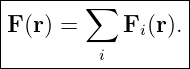
Newtonian gravity is linear in the source masses. If several masses are present, the net
gravitational force is the vector sum of the individual forces.
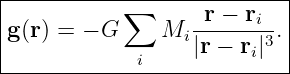
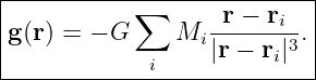
For a test mass m at position r and source masses Mi at positions ri,
The contribution from source i is
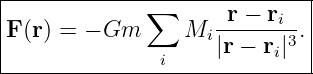
Therefore
Dividing by the test mass gives the gravitational field:
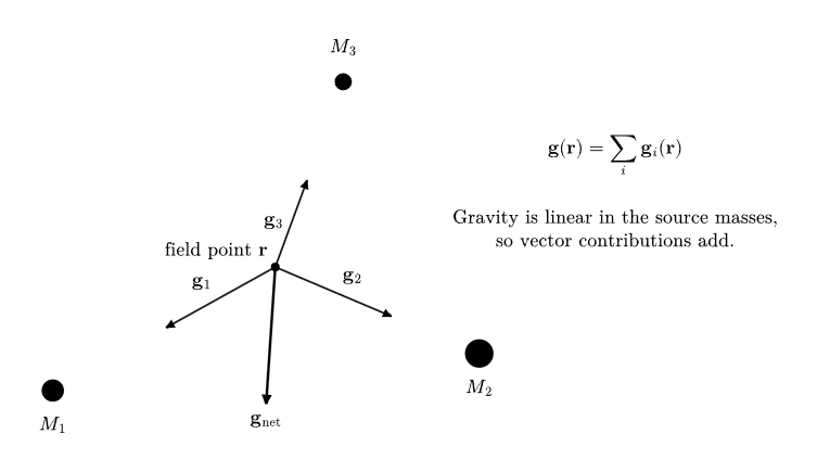
Figure. For several gravitating sources, each mass contributes a vector field at the
observation point. The net Newtonian gravitational field is their vector sum.
This superposition principle is the starting point for the Newtonian N-body equations developed
much later in the series.
13 A two-source example on one line
Consider two equal source masses M fixed at
At the midpoint x = 0, the left mass produces a field of magnitude
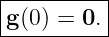
pointing left, while the right mass produces the same magnitude pointing right. Therefore
Zero net field does not mean gravity is absent. It means the individual contributions cancel at that
point.
The same distinction becomes important in multi-body celestial mechanics, where equilibrium
points arise from balances among several gravitational and inertial terms.
14 From discrete masses to a continuous mass distribution
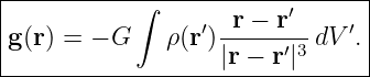
If matter is described by a mass density
then a small source volume dV ′ contains mass
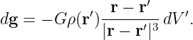
The field contribution at observation point r is
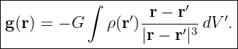
Integrating over the source gives
This equation extends the point-mass law to planets, stars, gas clouds, stellar systems, and galaxies
within Newtonian gravity.
Its direct evaluation can be difficult, but symmetry can simplify it dramatically.
15 Preview: spherical symmetry and the shell theorem
For a spherically symmetric body, Newton’s shell theorem gives two powerful results:
- outside a spherical shell, the gravitational field is exactly the same as if the shell’s mass
were concentrated at its center;
- inside an ideal thin spherical shell, the net gravitational field is zero.
Consequently, outside any spherically symmetric body of total mass M,
provided r lies outside the mass distribution.
This is why planets and stars can often be treated as point masses when studying external orbital
motion, even though they are physically extended objects.
The shell theorem and extended spherical distributions will be developed more fully
in CM02E1 when gravitational potential provides a particularly efficient route to the
calculation.
16 What the point-mass approximation really means
A body does not have to be physically tiny to behave gravitationally like a point mass.
For a spherically symmetric object, the external field is exactly equivalent to that of a point mass
at the center. For a nearly spherical body, the point-mass model is often the dominant term in a
more detailed gravitational-field expansion.
Thus the approximation
can be excellent even when the body’s physical radius is large, provided the observer is outside
the body and departures from spherical symmetry are unimportant for the required
accuracy.
Later perturbation theory will explicitly add nonspherical gravitational effects rather than hiding
them inside the ideal law.
17 Example 3: Earth acting on the Moon
Take the mean Earth–Moon separation as approximately
The acceleration produced by Earth at that distance is
| gE(rEM) | = G | (68)
|
| ≈ 2.70 × 10⁻³ m/s2. | (69) |
Thus
Using a lunar mass of approximately
the mutual force magnitude is approximately
Earth experiences exactly the same force magnitude in the opposite direction. Because Earth’s
mass is much larger, Earth’s acceleration toward the Moon is much smaller than the Moon’s
acceleration toward Earth.
This observation is the first hint that saying “the Moon orbits Earth” is an approximation. In the
exact two-body problem, both bodies move around their common center of mass.
18 Gravitational force is central
For a source at the origin,
The force is parallel or antiparallel to r. Therefore it is a central force.
The torque about the force center is
| τ | = r × F | (74)
|
| = r ×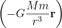 | (75)
|
| = 0. | (76) |
Thus
We will derive the consequences carefully later, but already we can preview one of the deepest
structural facts of celestial mechanics:
From that conservation law will come planar motion and Kepler’s equal-area law.
19 Preview: gravity is conservative
The Newtonian point-mass force also has the special property that it can be derived from a scalar
potential energy.
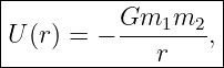
For two point masses,
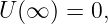
with the conventional choice
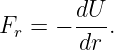
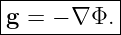
The radial force is recovered from
Indeed,
CM02 will develop gravitational potential and potential energy in detail, including the
relation
For now, the important preview is that Newtonian gravity conserves mechanical energy for an
isolated system.
20 Why the potential is negative
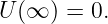
With the reference choice
two attracting masses at finite separation have
The negative sign encodes the fact that positive work must be supplied to separate a bound pair
from finite separation to infinity.
This sign will later become central to orbital classification:
That result belongs later in the sequence, after the kinetic and potential terms have been combined
correctly.
21 Astrophysical scale invariance of the same law
One of the remarkable features of Newtonian gravity is that the same mathematical law describes
systems across an enormous range of scale.
The same expression
is used to model, at the appropriate approximation level:
- a falling laboratory mass near Earth;
- the Earth–Moon interaction;
- planets orbiting the Sun;
- binary stars;
- stars orbiting a compact central mass;
- the pairwise forces in an N-body star-cluster calculation.
The objects and distances change by many orders of magnitude, but the Newtonian
force law keeps the same structure until relativistic or extended-mass effects become
important.
This universality is one reason celestial mechanics provides such a powerful bridge between
classical mechanics and astrophysics.
22 When Newtonian point-mass gravity is not enough
The simple law is foundational, but it is not universally sufficient.
Corrections or more detailed models may be required when:
- the source is significantly nonspherical and its multipole gravity matters;
- several bodies produce comparable gravitational accelerations;
- tidal effects depend on the spatial gradient of gravity across an extended body;
- mass distributions are continuous rather than point-like;
- velocities or gravitational fields become relativistically strong;
- nongravitational forces such as radiation pressure, drag, or thrust are important.
Celestial mechanics is therefore not about using the most complicated force model possible. It is
about selecting the simplest model that contains the physics relevant to the question.
23 A compact vector summary
For two point masses with
the gravitational force on body 2 due to body 1 is
The force on body 1 due to body 2 is
For a source mass M at the origin, the gravitational field is
The force on a test mass m is
For many point sources,
For a continuous density distribution,
These equations are the gravitational foundation for the rest of the celestial-mechanics
series.
24 Common mistakes
- Writing 1∕r3 in the vector law and concluding that gravity is an inverse-cube force.
The numerator contains the vector r, so the magnitude still scales as 1∕r2.
- Using a minus sign without defining the relative-position vector. The sign only has
meaning relative to a coordinate convention.
- Treating G and g as the same quantity. G is the universal gravitational constant; g is
a gravitational field or acceleration.
- Treating one body as fixed without checking the mass ratio. The exact two-body
problem allows both masses to move.
- Adding gravitational magnitudes instead of vectors when more than one source is
present.
- Assuming the inverse-square geometry alone proves Newton’s gravitational law. It
explains the spherical spreading structure but not the existence or strength of the
interaction.
- Applying the point-mass law inside an arbitrary extended body. The external
point-mass equivalence requires spherical symmetry; interior fields require integrating
the mass distribution or using symmetry results.
- Forgetting that a = g follows after dividing by the test mass. The gravitational force
itself is still proportional to the test mass.
25 What CM01 adds to the series
CM00 gave the roadmap. CM01 supplies the first dynamical law on which that roadmap
rests.
The main chain is
The key result for a point source is
The next companion entry, CM01E1, should turn this law into worked calculations involving force
ratios, surface gravity, two-body force pairs, vector superposition, and astronomical
scaling.
The next main theory article, CM02, will develop gravitational potential and potential energy from
the same inverse-square force and establish the conservative-field structure
References
[1] Bradley W. Carroll and Dale A. Ostlie, An Introduction to Modern Astrophysics, 2nd
ed., Pearson/Addison-Wesley, 2007.
[2] Herbert Goldstein, Charles Poole, and John Safko, Classical Mechanics, 3rd ed.,
Addison-Wesley, 2001.
[3] J. M. A. Danby, Fundamentals of Celestial Mechanics, 2nd ed., Willmann-Bell, 1988.
[4] Roger R. Bate, Donald D. Mueller, and Jerry E. White, Fundamentals of
Astrodynamics, Dover Publications, 1971.
[5] Carl D. Murray and Stanley F. Dermott, Solar System Dynamics, Cambridge
University Press, 1999.
[6] Isaac Newton, The Principia: Mathematical Principles of Natural Philosophy, trans.
I. Bernard Cohen and Anne Whitman, University of California Press, 1999.







![[F ] = kgm ∕s2,](https://images.physicslibrary.org/cache/objects/1249/make4ht/CelestialMechanicsNewtonsLawOfUniversalGravitation15x.png)
![3
[GM ] = m--.
s2](https://images.physicslibrary.org/cache/objects/1249/make4ht/CelestialMechanicsNewtonsLawOfUniversalGravitation19x.png)





![2
[g] = m/s .](https://images.physicslibrary.org/cache/objects/1249/make4ht/CelestialMechanicsNewtonsLawOfUniversalGravitation36x.png)