Calculus of Variations: Vector Trajectory Problems and Conserved Momentum
CV07 derived the Euler–Lagrange equations for several dependent variables, and CV07E1 used
them for coupled matrix systems. This companion set changes the geometric viewpoint. The
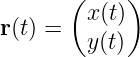
unknown is now a trajectory
in the plane, or more generally a vector curve in configuration space. The central questions
are:
- how a scalar action produces a vector differential equation;
- how fixed and free endpoint conditions act component by component;
- when generalized momentum is a conserved vector;
- how a spatial symmetry can conserve only selected momentum components;
- how endpoint freedom produces a geometric transversality condition.
These are the trajectory-level forms of the vector Euler–Lagrange equations used throughout
analytical mechanics [3, 4, 5]. The examples remain elementary enough that every stationary path
can be found in closed form.
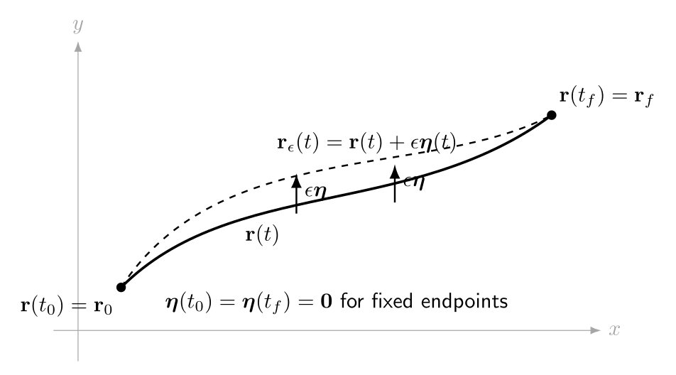
Figure. A vector trajectory and an admissible variation. With both endpoints fixed, the
perturbation vector must vanish at the initial and final times, while it may point in
arbitrary directions in the interior.
1 Formula sheet for this set
For
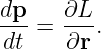
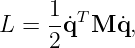
the vector first variation is [1, 2]
The generalized momentum vector is
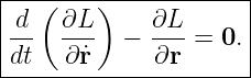
The vector Euler–Lagrange equation is therefore
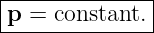
If the Lagrangian has no dependence on the position vector,
then
so the entire generalized momentum vector is conserved. If only one coordinate is absent from the
Lagrangian, only the corresponding momentum component is guaranteed to be conserved. This
is the finite-dimensional preview of the symmetry ideas developed systematically in
CV20.
Part I: Exercises
Exercise 1: vector Dirichlet energy and the straight path
Let
where
- Derive the vector Euler–Lagrange equation.
- Solve the resulting boundary-value problem.
- Show directly that the stationary path is also the unique global minimum of this
quadratic functional.
Exercise 2: a free particle and conservation of the momentum vector
For a particle of mass  , consider
with fixed endpoint positions  and
and  .
.
- Compute the generalized momentum vector.
- Use Euler–Lagrange to prove that this vector is conserved.
- Solve for the stationary trajectory joining the two endpoint events.
- Interpret the result geometrically.
Exercise 3: uniform gravity with two fixed endpoint events
Take
for  , with
- Derive the two Euler–Lagrange equations.
- Identify which momentum component is conserved and explain why.
- Solve the boundary-value problem explicitly.
- Show that the spatial trajectory is parabolic when
 .
.
Exercise 4: one cyclic spatial coordinate
Let
- Derive the Euler–Lagrange equations.
- Prove that
 is conserved.
- Explain why
 is not generally conserved.
- State the additional condition under which the full vector
 is conserved.
Exercise 5: a translation-invariant anisotropic kinetic energy
Let  and
and
where  is a constant symmetric positive-definite matrix. The endpoint positions are fixed at
 and
and  over an elapsed time
  .
.
- Find the generalized momentum vector.
- Prove that it is constant.
- Find the stationary path.
- Express the constant momentum in terms of
 ,
,  ,
,  , and
, and  .
.
Exercise 6: one fixed endpoint component and one free component
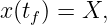
Suppose the initial position is fixed. At  , the final horizontal coordinate is prescribed,
but  is free. The final time is fixed.
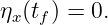
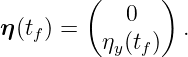
- State the allowed endpoint variation
 .
.
- Use the boundary term in
 to derive the natural endpoint condition.
- For the standard mechanical Lagrangian
interpret the endpoint condition physically.
Exercise 7: endpoint constrained to a target curve
The initial position and final time are fixed, but the final point may slide along a smooth target
curve  . Let
. Let  be a tangent vector to
  at the terminal point.
- Show that the allowed endpoint variation is tangent to
 .
.
- Derive
- If the target curve is represented by
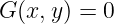 , show that
for some scalar  .
.
- For a free particle, explain the geometric meaning of the condition.
Exercise 8: a terminal endpoint cost
Let
where the initial position is fixed and the final position is free.
- Derive the terminal condition relating
 to
to  .
.
- For
write the terminal condition explicitly.
- Explain how the endpoint penalty changes the natural condition
 .
.
Exercise 9: momentum-vector conservation as a symmetry test
For a general planar Lagrangian
classify the momentum conservation implied by each case:
 is independent of
  but depends on
  .
.
 is independent of
  but depends on
  .
.
 is independent of both
  and
and  .
.
 depends on
  and
and  only through a central potential
 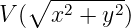 . Is the
linear momentum vector generally conserved?
. Is the
linear momentum vector generally conserved?
Part II: Complete worked solutions
Solution 1: vector Dirichlet energy and the straight path
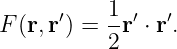
The integrand is
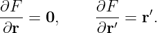
Therefore
The vector Euler–Lagrange equation gives
so
Integrating twice,
The endpoint conditions imply
Hence
This is the straight segment joining the two endpoint vectors.
To prove global minimality directly, write any admissible competitor as
where
Then
| J[r] | =  ∫
01∥r
∗′ + u′∥2ds ∫
01∥r
∗′ + u′∥2ds | (31)
|
| = J[r∗] + ∫
01r
∗′⋅ u′ds +  ∫
01∥u′∥2ds. ∫
01∥u′∥2ds. | (32) |
Because  is constant,
Thus
Equality requires  , and the endpoint conditions then force
  . Therefore the straight
path is the unique global minimizer.
. Therefore the straight
path is the unique global minimizer.
Solution 2: a free particle and conservation of the momentum vector
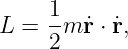
For
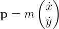
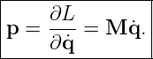
the generalized momentum is
The Lagrangian contains no  , so
, so
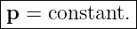
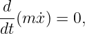
Euler–Lagrange therefore gives
Hence
For a constant mass,  is constant as well. Therefore
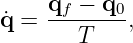
The stationary path in configuration space is a straight line traversed at constant velocity.
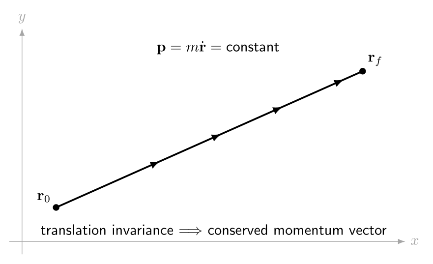
Figure. For a free particle the Lagrangian is invariant under spatial translation, so both
planar coordinates are cyclic and the entire momentum vector is constant. The trajectory
between fixed endpoint events is therefore straight with uniform velocity.
This is a simple but important example of a vector conservation law. The two component
equations
are equivalent to the single vector statement  .
.
Solution 3: uniform gravity with two fixed endpoint events
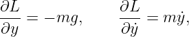
The Lagrangian is
For  ,
,
Thus
For  ,
,
so
or
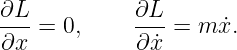
Since  is cyclic,
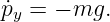
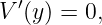
But  depends explicitly on
  , so
, so  is not conserved. Indeed,
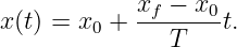
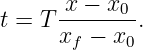
The horizontal solution satisfying the endpoints is
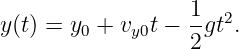
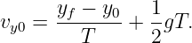
The vertical solution has the form
Imposing 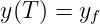 gives
gives
Therefore
If  , then
Substitution into  produces a quadratic polynomial in
  , so the spatial trajectory is a
parabola.
, so the spatial trajectory is a
parabola.
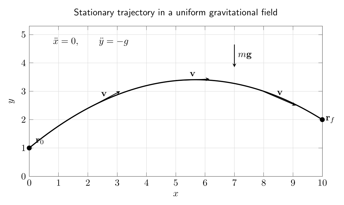
Figure. A stationary mechanical trajectory in a uniform gravitational field. Spatial
translation symmetry remains in the horizontal direction, giving constant  , while
gravity changes the vertical momentum.
, while
gravity changes the vertical momentum.
This exercise illustrates why conservation should be checked component by component before it is
promoted to a vector statement.
Solution 4: one cyclic spatial coordinate
For
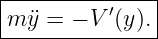
the  equation is
so
The  equation is
hence
Thus
which is generally nonzero.
The full vector momentum
is conserved only when the Lagrangian is independent of both  and
and  . For this example that
requires
. For this example that
requires
so the potential must be constant over the region of interest.
Solution 5: a translation-invariant anisotropic kinetic energy
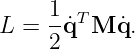
The Lagrangian is
Because  is symmetric,
There is no explicit dependence on  , so
, so
Since  is constant and nonsingular,
implies
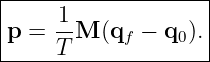
For an elapsed time  , the stationary path is
Its constant velocity is
so
The path is still affine in configuration space. The matrix  changes the relationship between
velocity and momentum, not the fact that both are constant for this translation-invariant
quadratic Lagrangian.
changes the relationship between
velocity and momentum, not the fact that both are constant for this translation-invariant
quadratic Lagrangian.
Solution 6: one fixed endpoint component and one free component
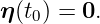
At the initial time,
At the final time, 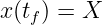 is fixed, so
The final  value is free, so
  is arbitrary. Thus
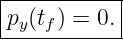
After the interior Euler–Lagrange equations are satisfied, the remaining endpoint term
is
Because  is arbitrary,
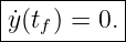
For
we have  , hence
The final velocity has no component along the direction in which the endpoint is free
to move. This is the componentwise natural boundary condition derived abstractly in
CV05.
Solution 7: endpoint constrained to a target curve
Let  lie on a smooth target curve
  . The endpoint may move along the curve but
not away from it. Therefore an admissible first-order endpoint displacement has the
form
. The endpoint may move along the curve but
not away from it. Therefore an admissible first-order endpoint displacement has the
form
where  is tangent to
  and
and  is arbitrary.
The endpoint contribution to the first variation is
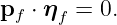
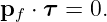
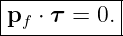
Stationarity for every allowed  requires
Thus the terminal momentum is normal to the target curve.
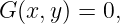
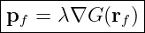
If the curve is defined by
then  is normal to the curve. Consequently
for some scalar  .
.
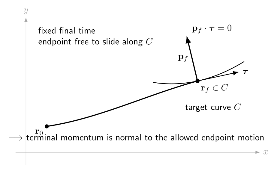
Figure. At a fixed final time, a terminal point constrained to a curve may vary only along
the curve tangent. The variational endpoint term therefore forces the terminal generalized
momentum to be normal to every allowed endpoint motion.
For a free particle,  , so the terminal velocity is normal to
  . In the Euclidean
kinetic-energy problem this reproduces the familiar orthogonality of a shortest path to a freely
chosen point on a target curve.
. In the Euclidean
kinetic-energy problem this reproduces the familiar orthogonality of a shortest path to a freely
chosen point on a target curve.
Solution 8: a terminal endpoint cost
Consider
The variation of the terminal cost is
After imposing the interior Euler–Lagrange equations and the fixed initial endpoint, the terminal
part of the first variation is
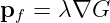
Because the final position is completely free, all components of  are arbitrary. Hence
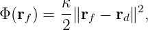
For the quadratic terminal penalty
we have
Therefore
Without a terminal cost, a completely free endpoint would give  . The endpoint penalty
replaces that zero-momentum condition by a balance between terminal momentum
and the gradient of the endpoint objective. This structure later reappears in optimal
control.
. The endpoint penalty
replaces that zero-momentum condition by a balance between terminal momentum
and the gradient of the endpoint objective. This structure later reappears in optimal
control.
Solution 9: momentum-vector conservation as a symmetry test
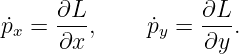
The component Euler–Lagrange equations are
Therefore:
- If
 is independent of
  , then
but  need not be constant.
- If
 is independent of
  , then
but  need not be constant.
- If
 is independent of both
  and
and  , then
The full translation group acts as a symmetry of the Lagrangian.
- For a central potential
the Lagrangian depends on position, so the linear momentum vector is not generally
conserved. The force points radially and changes the momentum vector. Rotational
symmetry instead leads to angular-momentum conservation, a result developed
systematically through Noether’s theorem in CV20 [4, 5].
2 A compact endpoint-condition map for vector trajectories
For a stationary vector trajectory, the boundary contribution at a fixed final time is
The allowed endpoint motion determines the terminal condition:
|
|
|
Endpoint freedom | Allowed variation | Stationarity condition |
|
|
|
Fully fixed | 
| no additional natural
condition |
All components free | arbitrary  | 
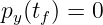
|
Only  free free | 
| 
|
Constrained to curve  | tangent to  | 
|
Free with terminal cost  | arbitrary  | 
|
|
|
|
The important lesson is that a vector endpoint condition is not usually imposed all at once. Each
free direction contributes one scalar transversality condition.
3 Common mistakes
- Mistake: treating
 as conserved whenever one coordinate is cyclic. A single cyclic
coordinate conserves one momentum component, not necessarily the entire vector.
as conserved whenever one coordinate is cyclic. A single cyclic
coordinate conserves one momentum component, not necessarily the entire vector.
- Mistake: forgetting that fixed endpoint values make the corresponding components
of
 vanish.
- Mistake: setting every terminal momentum component to zero when the endpoint is
constrained to a curve. Only momentum components along allowed endpoint directions
must vanish.
- Mistake: assuming that a conserved generalized momentum is always
 . For a
general Lagrangian it is
. For a
general Lagrangian it is  .
.
- Mistake: confusing the stationary mechanical trajectory with a shortest spatial path.
Hamilton’s action and Euclidean path length are different functionals.
- Mistake: using Euler–Lagrange stationarity alone as a proof of global minimality.
Exercise 1 admits a direct positivity proof, but general mechanical actions need not be
minima.
4 Summary
For a vector trajectory  , the Euler–Lagrange equation may be written
The generalized momentum vector is
If every spatial coordinate is cyclic, then
If only selected coordinates are cyclic, only the corresponding momentum components are
conserved.
At a fixed terminal time, endpoint freedom is encoded in
A completely free endpoint gives  ; a point constrained to a curve forces
  normal to
that curve; and a terminal cost changes the condition to
normal to
that curve; and a terminal cost changes the condition to
CV07E2 therefore ties together vector Euler–Lagrange equations, trajectory geometry,
conservation laws, and the endpoint conditions introduced in CV05. The next main
lesson, CV08, increases the differential order of the functional and shows how repeated
integration by parts creates higher-order Euler–Lagrange equations and additional boundary
terms.
References
[1] I. M. Gelfand and S. V. Fomin, Calculus of Variations, Dover Publications, 2000.
[2] Bruce van Brunt, The Calculus of Variations, Springer, 2004.
[3] Cornelius Lanczos, The Variational Principles of Mechanics, 4th ed., Dover
Publications, 1986.
[4] Herbert Goldstein, Charles Poole, and John Safko, Classical Mechanics, 3rd ed.,
Addison-Wesley, 2002.
[5] V. I. Arnold, Mathematical Methods of Classical Mechanics, 2nd ed., Springer, 1989.

![[parent]](https://images.physicslibrary.org/images/uparrow.png)
![∫ t
f ˙
S [r] = t0 L(t,r,r)dt,](https://images.physicslibrary.org/cache/objects/1204/make4ht/CalculusOfVariationsVectorTrajectoryProblemsAndConservedMomentum1x.png)
![∫ tf [∂L d ( ∂L ) ] [∂L ]tf
δS = --- − -- --- ⋅ η dt + --- ⋅ η .
t0 ∂r dt ∂r˙ ∂˙r t0](https://images.physicslibrary.org/cache/objects/1204/make4ht/CalculusOfVariationsVectorTrajectoryProblemsAndConservedMomentum2x.png)



![1 ∫ 1
J [r] = -- ∥r ′(s)∥2ds,
2 0](https://images.physicslibrary.org/cache/objects/1204/make4ht/CalculusOfVariationsVectorTrajectoryProblemsAndConservedMomentum7x.png)

![∫ tf1
S [r] = --m ∥˙r∥2dt
t0 2](https://images.physicslibrary.org/cache/objects/1204/make4ht/CalculusOfVariationsVectorTrajectoryProblemsAndConservedMomentum10x.png)




![∫
tf
J [r] = L (t,r,r˙) dt + Φ (r(tf)),
t0](https://images.physicslibrary.org/cache/objects/1204/make4ht/CalculusOfVariationsVectorTrajectoryProblemsAndConservedMomentum45x.png)








![∫
1 ′ ′
r∗ ⋅ u ds = (B − A ) ⋅ [u(1) − u(0)] = 0.
0](https://images.physicslibrary.org/cache/objects/1204/make4ht/CalculusOfVariationsVectorTrajectoryProblemsAndConservedMomentum76x.png)
![1 ∫ 1
J[r] − J [r∗] =-- ∥u ′∥2ds ≥ 0.
2 0](https://images.physicslibrary.org/cache/objects/1204/make4ht/CalculusOfVariationsVectorTrajectoryProblemsAndConservedMomentum77x.png)












![-d ′
dt(m y˙) − [− V (y)] = 0,](https://images.physicslibrary.org/cache/objects/1204/make4ht/CalculusOfVariationsVectorTrajectoryProblemsAndConservedMomentum119x.png)








![∫
tf
J[r] = L dt + Φ (rf).
t0](https://images.physicslibrary.org/cache/objects/1204/make4ht/CalculusOfVariationsVectorTrajectoryProblemsAndConservedMomentum166x.png)

![[pf + ∇ Φ (rf)] ⋅ ηf.](https://images.physicslibrary.org/cache/objects/1204/make4ht/CalculusOfVariationsVectorTrajectoryProblemsAndConservedMomentum168x.png)