Work by Variable Forces
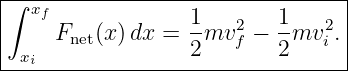
For a constant force, M03-01 established the familiar result
That formula is a special case. When the force changes in magnitude, direction, or both as the
particle moves, the displacement must be divided into sufficiently small pieces and the work
contributions added.
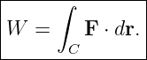
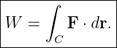
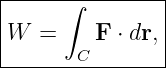
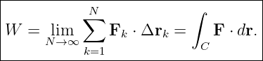
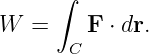
The general definition is the line integral
where C is the actual path followed by the particle.
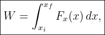
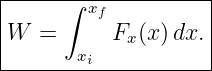
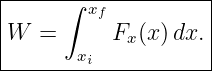
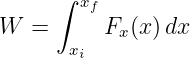
In one-dimensional motion along the x axis, this reduces to
This article develops the meaning and use of that integral, connects it to the signed area under a
force-position graph, applies it to springs and piecewise forces, and shows why the path itself can
matter in more than one dimension.

Figure 1. Constant-force work is the special case in which every small displacement experiences
the same force. For a variable force, the total work is obtained by summing differential
contributions dW = F ⋅ dr.
1 From a finite sum to an integral
Suppose a particle moves from position ri to rf along a path C. Divide the path into many short
displacement vectors
If each segment is sufficiently short, the force over that segment can be approximated by a nearly
constant value Fk. The work on segment k is approximately
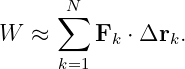
Adding all segments,
In the limit of increasingly fine subdivisions,
Thus the work integral is the continuum limit of ordinary constant-force work.
2 Differential work
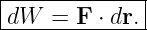
The differential amount of work associated with an infinitesimal displacement dr is
If 𝜃 is the instantaneous angle between F and dr, then
where ds = |dr| is the infinitesimal path length.
Therefore:
- dW > 0 if the force has a component along the displacement,
- dW = 0 if the force is perpendicular to the displacement,
- dW < 0 if the force has a component opposite the displacement.
The total work is obtained by integrating these signed contributions.
3 One-dimensional variable force
For motion along the x axis,
If
then
Hence
This result should be interpreted carefully. The integration variable x carries a sign
through dx. If the particle moves toward decreasing x, then dx < 0 along that part of the
motion.
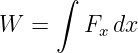
4 Force-position graphs and signed area
The integral
has a direct geometric interpretation.
On a graph of Fx versus x:
- area above the x axis contributes positive work,
- area below the x axis contributes negative work,
- the net signed area equals the total work.
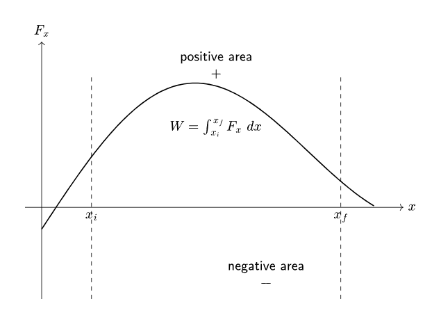
Figure 2. The work done by a one-dimensional variable force equals the signed area under the Fx
versus x curve between the initial and final positions.
Because
the area under a force-position graph has units
5 Example 1: a quadratic force law
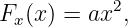
Suppose
where a is a constant.
The work from x = 0 to x = L is
| W | = ∫
0Lax2 dx | (18)
|
| = a![[ 3]
x--
3](https://images.physicslibrary.org/cache/objects/1375/make4ht/WorkByVariableForces17x.png) 0L 0L | (19)
|
| =  . . | (20) |
A common mistake would be to multiply the final force aL2 by the distance L. That would give
aL3, which is three times too large. The force varies throughout the motion, so the integral is
required.
6 Average force in one dimension
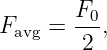
For motion from xi to xf, define an average force over the interval by
Then
This is useful when the force-position curve is simple enough that its average value is
obvious.
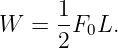
For example, if Fx increases linearly from 0 to F0 over a displacement L, then
so
This is the area of a triangle.
7 Piecewise variable forces
Many problems specify a force graph made of straight-line or constant segments. The easiest
method is often geometric area rather than direct integration.
Consider the force-position graph in Figure 3.
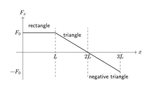
Figure 3. A piecewise force-position graph. The total work is the sum of the signed geometric
areas of the rectangle, triangle, and negative triangle.
Suppose the graph contains:
- a constant force +F0 from x = 0 to x = L,
- a linear decrease from +F0 at x = L to 0 at x = 2L,
- a linear decrease from 0 at x = 2L to −F0 at x = 3L.
The three signed areas are
| W1 | = F0L, | (25)
|
| W2 | =  F0L, F0L, | (26)
|
| W3 | = − F0L. F0L. | (27) |
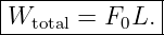
Therefore
The positive and negative triangular contributions cancel.
8 Spring force
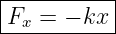
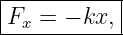
An ideal spring obeys Hooke’s law:
where x is the displacement from equilibrium and k is the spring constant.
The negative sign means that the spring force points opposite the displacement.
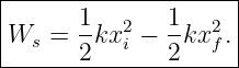
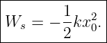
The work done by the spring as its endpoint moves from xi to xf is
| Ws | = ∫
xixf
(−kx) dx | (30)
|
| = −k![[ ]
x2
2--](https://images.physicslibrary.org/cache/objects/1375/make4ht/WorkByVariableForces27x.png) xixf
. xixf
. | (31) |
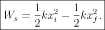
Thus
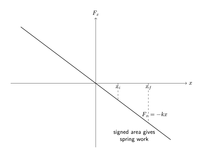
Figure 4. For Fx = −kx, the work done by the spring between two positions is the signed area
under the straight-line force-position graph.
Several special cases are important.
8.1 Spring released from extension x0 to equilibrium
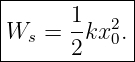
Set
Then
The spring does positive work while moving toward equilibrium.
8.2 Stretching from equilibrium to x0
Set
Then
The spring does negative work because its force opposes the outward displacement.
9 Work done by an external agent on a spring
If a spring is stretched very slowly so that the endpoint is approximately in mechanical equilibrium
throughout the process, the external applied force is
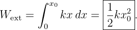
The work done by the external agent in stretching from 0 to x0 is
This has the same magnitude as the negative work done by the spring:
The distinction between “work done by the spring” and “work done on the spring” is
essential.
10 Using variable-force work with the work-energy theorem
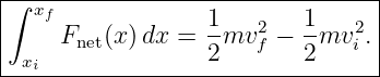
M03-02 established
If the net force varies with position in one dimension,
This relation often determines speed without solving for acceleration as a function of
time.
11 Example 2: speed under a linearly increasing net force
A 2.0 kg particle starts from rest at x = 0. The net force is
with F in newtons when x is in meters.
Find the speed at x = 3.0 m.
The net work is
| Wnet | = ∫
034xdx | (43)
|
| = ![[2x2]](https://images.physicslibrary.org/cache/objects/1375/make4ht/WorkByVariableForces39x.png) 03
03 | (44)
|
| = 18 J. | (45) |
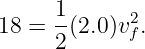
From the work-energy theorem,
Therefore
12 Parameterized paths in several dimensions
In more than one dimension, the work integral is
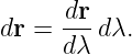
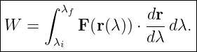
A convenient way to evaluate it is to parameterize the path using a variable λ:
Then
Therefore
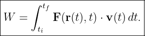
If time itself is used as the parameter,
so
This form remains valid even if the force depends explicitly on time.
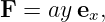
13 Example 3: work along a two-dimensional path
Let
where a is a constant.
Suppose the particle moves from (0, 0) to (L,L) along two different paths.
13.1 Path A: first along x, then along y
Along the first segment,
so
Hence
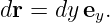
Along the vertical segment,
Since F points in the x direction,
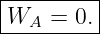
Therefore
13.2 Path B: first along y, then along x
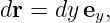
Along the first vertical segment,
so the work is again zero.
Along the top horizontal segment,
and
Thus
| WB | = ∫
0LaLdx | (64)
|
| = aL2 . | (65) |
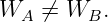
The same endpoints give different work:
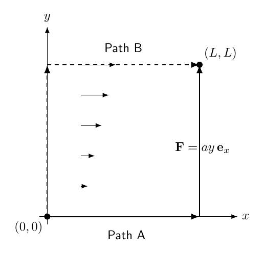
Figure 5. For the field F = ay ex, the work from (0,0) to (L,L) depends on the path. Path A
gives zero work, while Path B gives aL2.
This example demonstrates path-dependent work. A later mechanics article will develop the special
class of forces for which the work depends only on the endpoints.
14 Reversing a path
For a force field that is evaluated along the same geometric path in reverse order,
Therefore
This sign reversal is a direct consequence of the line integral.
For example, an ideal spring does positive work while returning from x0 to equilibrium and
negative work while being stretched from equilibrium to x0.
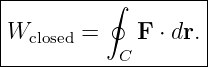
15 Work around a closed path
If a particle returns to its starting point, the path is closed. The work is written
A closed path does not automatically imply zero work. The result depends on the force
field.
For the path-dependent example
one can construct a rectangular closed loop for which the total work is nonzero.
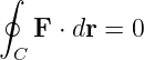
The conditions under which
for every closed path will be developed later with conservative forces and potential
energy.
16 Units and dimensional checks
The work integral
has dimensions
Since
we obtain
For a spring,
so
Then
which confirms the dimensions of
17 Common mistakes
- Using W = FΔx when the force varies substantially with position.
- Using the final force instead of integrating over the full interval.
- Forgetting that area below the axis on an Fx versus x graph contributes negative work.
- Confusing area under an F versus x graph with area under an F versus t graph.
- Forgetting that ∫
Fx dx has units of joules, while ∫
Fx dt has units of impulse.
- Dropping the minus sign in Hooke’s law Fx = −kx.
- Confusing work done by a spring with work done on a spring.
- Assuming that the work between two points is always independent of path.
- Evaluating a multidimensional line integral without first specifying the path.
- Forgetting that reversing the path reverses the sign of the work along that same path.
18 Practice exercises
- A force varies as Fx = 3x2 in SI units. Find the work from x = 1 m to x = 4 m.
- A force increases linearly from 2 N at x = 0 to 10 N at x = 4 m. Find the work
geometrically and by integration.
- The force-position graph is a triangle above the axis with base 6 m and height 12 N.
Find the work.
- The force-position graph contains +20 J of positive signed area and −7 J of negative
signed area. Find the net work.
- A spring with k = 300 N∕m is stretched from x = 0.10 m to x = 0.25 m. Find the work
done by the spring.
- For the same spring, find the work done by an external agent during a slow stretch
from x = 0 to x = 0.25 m.
- A 1.0 kg particle starts from rest and experiences a net force Fx = 6x from x = 0 to
x = 2.0 m. Find its final speed.
- Parameterize the straight-line path from (0, 0) to (L,L) as r(λ) = λLex + λLey,
0 ≤ λ ≤ 1. Evaluate the work for F = ay ex.
- For F = ay ex, calculate the work around the rectangular loop (0, 0) → (L, 0) →
(L,H) → (0,H) → (0, 0).
- Explain why the area under an Fx versus x graph represents work but the area under
an Fx versus t graph does not.
19 Summary
For a variable force, work is defined by the line integral
In one-dimensional motion,
which equals the signed area under the force-position curve.
For an ideal spring,
and
Combined with the work-energy theorem,
In several dimensions, the path must be specified:
The next article, M03-04, develops power as the rate at which work is done.
References
References
[1] J. R. Taylor, Classical Mechanics, University Science Books, 2005.
[2] D. Kleppner and R. Kolenkow, An Introduction to Mechanics, 2nd ed., Cambridge
University Press, 2014.
[3] H. D. Young and R. A. Freedman, University Physics with Modern Physics, 15th ed.,
Pearson, 2020.
[4] OpenStax, University Physics, Volume 1, Rice University, 2016.








![[W ] = [F][x],](https://images.physicslibrary.org/cache/objects/1375/make4ht/WorkByVariableForces14x.png)




















![[W ] = [F][x].](https://images.physicslibrary.org/cache/objects/1375/make4ht/WorkByVariableForces65x.png)
![[F ] = M LT −2,](https://images.physicslibrary.org/cache/objects/1375/make4ht/WorkByVariableForces66x.png)
![2 −2
[W ] = M L T .](https://images.physicslibrary.org/cache/objects/1375/make4ht/WorkByVariableForces67x.png)

![[k] = F- = N ∕m.
x](https://images.physicslibrary.org/cache/objects/1375/make4ht/WorkByVariableForces69x.png)
![2 N 2
[kx ] = m-m = N m = J,](https://images.physicslibrary.org/cache/objects/1375/make4ht/WorkByVariableForces70x.png)