Strapdown Inertial Navigation Examples: Rotating-Frame Derivatives, Coriolis, and Centrifugal
Acceleration
This companion to INS02 develops rotating-frame kinematics through explicit calculations. The
goal is to make the transport theorem operational while preserving its physical meaning. The
reader should be able to look at each term in
and explain where it came from, what direction it points, and whether it belongs to an
inertial acceleration decomposition or to an apparent-force description in the rotating
frame.
Throughout this companion, the angular-acceleration vector is denoted by α = dω∕dt to keep the
rotating-frame notation compact.
The exercises are stated first so the article can be used as a self-study problem set. Complete
worked solutions follow. The notation follows INS02 and standard inertial-navigation texts: i
denotes an inertial frame, r a generic rotating frame, and ωir the angular velocity of r relative to i
[1, 2, 3].
1 Exercises
Exercise 1: An inertially fixed vector seen from rotating axes
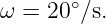
A frame r rotates counterclockwise about the common z axis relative to inertial frame i at the
constant rate
At t = 0 the frames are aligned. The physical vector
is fixed in inertial space.
At t = 3.0 s:
- find the rotation angle of frame r;
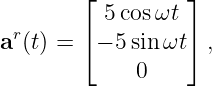
- compute the components ar;
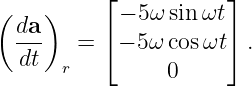
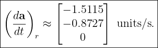
- differentiate those rotating-frame components directly with respect to time;
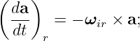
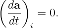
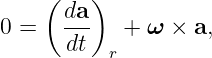
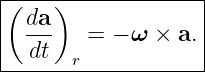
- verify the transport-theorem prediction
- explain why a vector can have a nonzero derivative of its coordinates in r even though its
inertial derivative is zero.
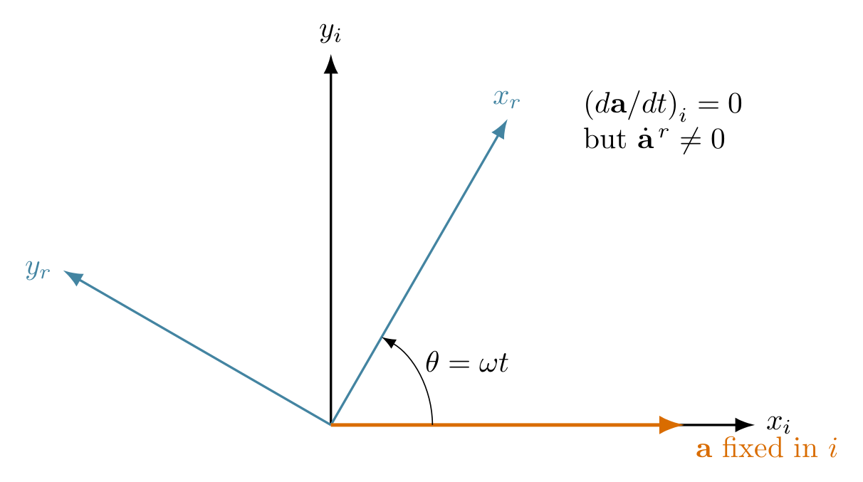
Figure. A physical vector fixed in inertial space acquires changing numerical components
in a rotating basis.
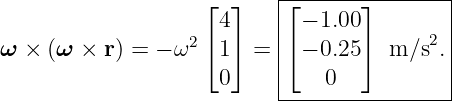
Exercise 2: A point fixed on a rotating turntable
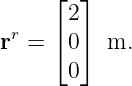
A point is rigidly attached to a horizontal turntable at
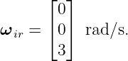
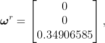
The turntable rotates at constant angular velocity
The origins coincide and the point is stationary relative to the turntable.
- Compute the inertial velocity of the point.
- Compute its inertial acceleration.
- Show that the acceleration is directed toward the rotation axis.
- If Newton’s law is instead written in rotating-frame form, what apparent centrifugal
acceleration is introduced?
Exercise 3: Radial motion and Coriolis acceleration
On a turntable rotating with
a small slider is instantaneously located at
and moves radially outward with rotating-frame velocity
At that instant its rotating-frame relative acceleration is zero, and the turntable rate is
constant.
- Compute the Coriolis term 2ω × vr.
- Compute the rotational centripetal term ω × (ω × r).
- Determine the total inertial acceleration.
- Compute its magnitude and direction in the xy plane.
- State the sign of the corresponding apparent Coriolis acceleration when Newton’s law
is rearranged into rotating-frame form.
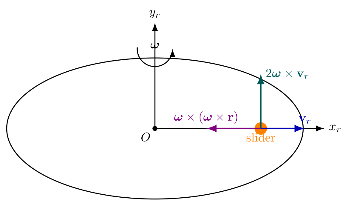
Figure. Radial motion on a rotating turntable. The Coriolis contribution is transverse to
the radial velocity while the rotational centripetal contribution points inward.
Exercise 4: Angular acceleration and the Euler term
A rigid arm rotates about the z axis. At one instant,
A point is fixed to the arm at
- Compute the Euler acceleration α× r.
- Compute the rotational centripetal acceleration.
- Find the total inertial acceleration of the point.
- Explain physically why the Euler and centripetal contributions are perpendicular in
this geometry.
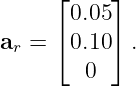
Exercise 5: Translating and rotating origin
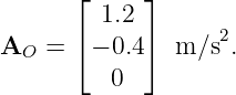
A moving coordinate frame r has an origin whose inertial acceleration is
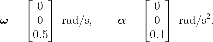
At a particular instant the frame has
A particle has rotating-frame state
Use
to compute every contribution separately and then the total inertial acceleration.
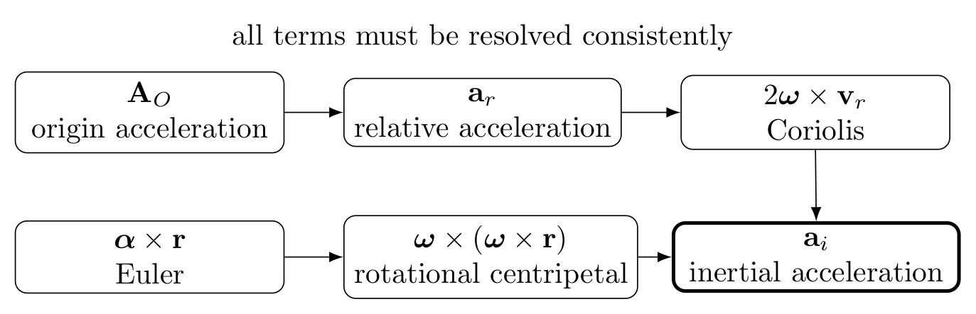
Figure. For a translating and rotating frame, inertial acceleration is assembled from origin
acceleration, relative acceleration, Coriolis, Euler, and rotational centripetal contributions.
Exercise 6: A point fixed to the rotating Earth is not inertially stationary
Approximate the Earth as a sphere of equatorial radius
rotating at
Consider a point fixed to the Earth at the equator.
- Compute its inertial speed due solely to Earth rotation.
- Compute the magnitude of its rotational centripetal acceleration.
- Compare this acceleration with g = 9.81 m/s2 as a percentage.
- Explain why an Earth-fixed navigation frame is non-inertial even for an object that is
stationary in ECEF coordinates.
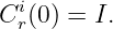
Exercise 7: DCM derivative from angular velocity
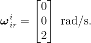
At t = 0, frames r and i are aligned. Frame r rotates relative to i with
Use the INS02 identity
to answer the following.
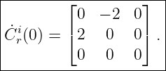
- Compute Ċri(0).
- Use a single forward-Euler step with Δt = 0.01 s to approximate Cri(Δt).
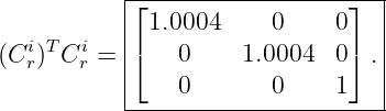
- Compute (Cri)T C
ri for that Euler approximation.
- Explain why ordinary Euler integration slowly destroys exact orthogonality.
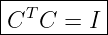
- Show analytically that if Ċ = ΩC with ΩT = −Ω, then the exact solution preserves
CT C = I.
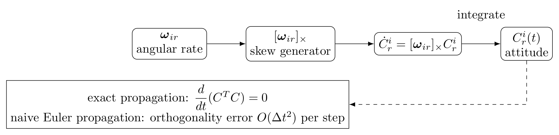
Figure. Angular velocity generates the time derivative of the DCM. Exact rotational
propagation remains on SO(3); a naive Euler step does not.
Exercise 8: Adding angular rates through nested frames
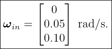
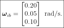
At one instant, frames i, e, n, and b are momentarily aligned so that all angular-rate components
can be added directly without another coordinate transformation. Suppose
in rad/s.
- Compute ωin.
- Compute ωib.
- Explain why this simple component-wise addition would generally be invalid if the
rates were supplied in different resolving frames.
- Relate the result to the later strapdown identity
Exercise 9: Inertial terms versus apparent accelerations
At some instant a particle is described in a uniformly rotating frame by
Assume the particle is force-free in the inertial frame, so ai = 0.
- Starting from the acceleration transport equation, solve for ar.
- Identify the apparent centrifugal acceleration.
- Identify the apparent Coriolis acceleration.
- Explain why their signs are opposite those of the corresponding terms in the inertial
acceleration decomposition.
Exercise 10: Implementation sanity check – degrees are not radians
A software routine evaluates the rotational centripetal magnitude using
The physical angular speed is 15∘∕s and the radius is r = 1.2 m. A programmer accidentally passes
the number 15 directly into a routine that expects rad/s.
- Compute the correct angular speed in rad/s.
- Compute the correct centripetal acceleration.
- Compute the erroneous acceleration produced by the software.
- By what factor is the result wrong?
- Propose at least three unit tests or interface safeguards that could catch this class of
error in an inertial-navigation code base.
2 Worked solutions
Solution 1: An inertially fixed vector seen from rotating axes
The angular speed in SI units is
After 3 s,
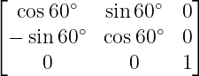
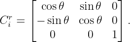
For axes rotated counterclockwise through 𝜃, the passive transformation from inertial coordinates
to rotating coordinates is
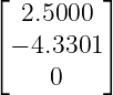
Thus
| ar | = C
irai | (25)
|
| =   | (26)
|
| =  . . | (27) |
Because
direct differentiation gives
At t = 3 s,
Now use the transport theorem. Since a is fixed in inertial space,
Therefore
so
Resolved in r,
and
| −ω × a | = −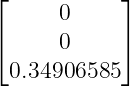 × ×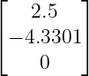 | (35)
|
| ≈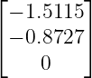 , , | (36) |
which agrees with the direct differentiation.
The physical vector has not changed. Only the basis vectors used to report its coordinates have
changed. A derivative of coordinate numbers is therefore not automatically the derivative of the
physical vector itself.
Solution 2: A point fixed on a rotating turntable
Because the point is fixed in r,
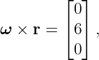
The inertial velocity is
| vi | = ω × r | (38)
|
| =  × × | (39)
|
| =  m/s. m/s. | (40) |
For constant ω,
First,
then
The acceleration is inward, toward the axis. Its magnitude is also
When Newton’s law is rearranged to describe dynamics in the rotating frame, the corresponding
apparent centrifugal acceleration is the negative of the rotational centripetal term:
It points outward.
Solution 3: Radial motion and Coriolis acceleration
The Coriolis contribution to inertial acceleration is
| 2ω × vr | = 2(2ez) × (1.5ex) | (47)
|
| = 6ey m/s2. | (48) |
The rotational centripetal term is
| ω × (ω × r) | = −ω2r | (49)
|
| = −(2)2(2e
x) | (50)
|
| = −8ex m/s2. | (51) |
Since ar = 0 and α = 0,
Its magnitude is
Measured counterclockwise from the positive x axis, the vector lies in quadrant II:
In rotating-frame Newton equations the apparent Coriolis term has the opposite sign:
This sign change is caused by algebraic rearrangement, not by a different cross-product
convention.
Solution 4: Angular acceleration and the Euler term
The Euler term is
| α× r | = (0.8ez) × (3ex) | (56)
|
| = 2.4ey m/s2. | (57) |
The rotational centripetal term is
so
The point is fixed to the rotating arm, so vr = ar = 0. Therefore
Its magnitude is
The Euler term is tangential because it results from changing angular speed. The centripetal term
is radial because it results from changing the direction of the tangential velocity. Hence they are
perpendicular for planar rotation about a fixed axis.
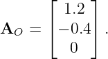
Solution 5: Translating and rotating origin
Evaluate the terms one at a time.
The origin contribution is already given:
The relative acceleration is
For the Coriolis term,
| 2ω × vr | = 2 × × | (64)
|
| =  m/s2. m/s2. | (65) |
For the Euler term,
| α× r | =  × × | (66)
|
| =  m/s2. m/s2. | (67) |
For the rotational centripetal contribution,
Adding all five terms,
| ai | =  + +  + +  + +  + +  | (69)
|
| =  m/s2. m/s2. | (70) |
This example is useful because no single term dominates by assumption. The inertial result
emerges only after all kinematic contributions are assembled consistently.
Solution 6: A point fixed to the rotating Earth is not inertially stationary
At the equator, the perpendicular distance to the Earth’s spin axis is approximately RE. The
inertial tangential speed is therefore
| v | = ωieRE | (71)
|
| = (7.292115 × 10⁻⁵)(6.378137 × 10⁶) | (72)
|
| ≈ 465.10 m/s. | (73) |
The rotational centripetal acceleration is
| ac | = ωie2R
E | (74)
|
| ≈ 0.03392 m/s2. | (75) |
Relative to g = 9.81 m/s2,
Thus a point whose ECEF coordinates never change still travels around the Earth’s spin axis at
hundreds of meters per second in inertial space. ECEF is therefore a rotating, non-inertial
frame. This is precisely why Earth-rate and rotational terms enter terrestrial inertial
navigation.
Solution 7: DCM derivative from angular velocity
At t = 0,
The skew matrix is
Therefore
A forward-Euler step gives
| Cri(Δt) | ≈ I + Ċ
ri(0)Δt | (80)
|
| = 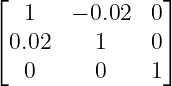 . . | (81) |
Now
The matrix is already slightly non-orthogonal after one Euler step. Repeated steps accumulate this
defect unless the integration method respects rotational geometry or the matrix is periodically
re-orthonormalized.
For the exact differential equation
consider
 (CT C) (CT C) | = ĊT C + CT Ċ | (84)
|
| = (ΩC)T C + CT (ΩC) | (85)
|
| = CT ΩT C + CT ΩC | (86)
|
| = CT (ΩT + Ω)C | (87)
|
| = 0. | (88) |
Thus if CT C = I initially,
for all time in the exact solution.
Solution 8: Adding angular rates through nested frames
Angular velocity obeys the relative-rate chain rule. At the instant when the frames are
aligned,
Hence
Similarly,
so
The geometric angular-velocity vectors may always be added in this way, but their numerical
coordinate columns may only be added after being resolved in a common frame. If, for example,
ωie were supplied in ECEF coordinates and ωnb in body coordinates, one or both would have to be
transformed first.
This is the conceptual origin of the later navigation-frame rate
Solution 9: Inertial terms versus apparent accelerations
For constant ω and a common origin,
Because the particle is force-free in inertial space,
Therefore
From Exercise 3,
and
Thus
The apparent centrifugal acceleration is
The apparent Coriolis acceleration is
Their signs are opposite because the transport equation first expresses inertial acceleration as a
sum of kinematic contributions. To write Newton’s law as an equation for ar, those contributions
are moved to the other side of the equation. The minus signs are therefore produced by
rearrangement.
Solution 10: Implementation sanity check – degrees are not radians
Convert the physical rate to radians per second:
The correct centripetal acceleration is
| ac | = ω2r | (104)
|
| = (0.2617994)2(1.2) | (105)
|
| ≈ 0.08225 m/s2. | (106) |
The erroneous implementation instead computes
The multiplicative error is
 | = 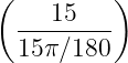 2 2 | (108)
|
| =  2 2 | (109)
|
| ≈ 3282.81. | (110) |
Useful safeguards include:
- require angular rates at software interfaces to use explicit SI-unit names such as
omega_rad_s;
- add a unit test using a known case such as ω = 1 rad/s and r = 1 m, for which ac = 1
m/s2;
- add a degrees-to-radians conversion test with 180∘∕s = π rad/s;
- assert physically plausible rate bounds at interfaces where such bounds are known;
- compare the cross-product implementation ω × (ω × r) against the scalar −ω2r
⊥ for
simple perpendicular test vectors;
- keep configuration files and telemetry metadata explicit about units rather than relying
on comments or convention.
In inertial navigation, unit errors can enter inside repeated integrations and therefore become
enormous state errors. Unit discipline is part of the physics implementation, not merely software
style.
3 What these exercises establish
The examples above reinforce several results that will be reused throughout the strapdown
series:
- A changing coordinate column does not necessarily imply a changing physical vector.
- A point fixed in a rotating frame generally has nonzero inertial velocity and
acceleration.
- Coriolis acceleration appears whenever there is relative motion in a rotating frame.
- Euler acceleration appears when the frame angular velocity changes.
- The term ω×(ω×r) is inward in the inertial acceleration decomposition; the outward
centrifugal term appears after rearranging Newton’s law in the rotating frame.
- A translating origin contributes its own inertial acceleration in addition to all rotational
terms.
- DCM kinematics are generated by a skew-symmetric angular-rate matrix, and exact
propagation preserves orthogonality.
- Angular-rate vectors from nested frames must be resolved in a common coordinate
frame before their component columns are added.
- Earth-fixed coordinates are non-inertial even when a vehicle is motionless relative to
the ground.
These points provide the mechanics foundation for INS03, where the measured accelerometer
quantity will be distinguished from ordinary kinematic acceleration.
References
[1] D. H. Titterton and J. L. Weston, Strapdown Inertial Navigation Technology, 2nd
ed., IET, 2004.
[2] P. D. Groves, Principles of GNSS, Inertial, and Multisensor Integrated Navigation
Systems, 2nd ed., Artech House, 2013.
[3] C. Jekeli, Inertial Navigation Systems with Geodetic Applications, Walter de Gruyter,
2001.
[4] H. Goldstein, C. Poole, and J. Safko, Classical Mechanics, 3rd ed., Addison-Wesley,
2002.

![[parent]](https://images.physicslibrary.org/images/uparrow.png)











![C˙ir = [ωiir]×Cir](https://images.physicslibrary.org/cache/objects/1347/make4ht/StrapdownInertialNavigationExamplesRotatingFrameDerivativesCoriolisAndCentrifugalAcceleration18x.png)










 m/s
m/s










![⌊0 − 2 0⌋
⌈ ⌉
[ω ]× = 2 0 0 .
0 0 0](https://images.physicslibrary.org/cache/objects/1347/make4ht/StrapdownInertialNavigationExamplesRotatingFrameDerivativesCoriolisAndCentrifugalAcceleration75x.png)