Motion Graphs in Kinematics

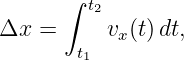
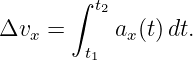
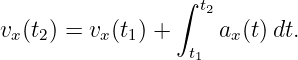
Motion graphs provide several complementary ways to describe the same motion. The most common are the position-time graph, velocity-time graph, and acceleration-time graph. They are connected by differentiation and integration:

v = dx, x dt

(1)

dvx- ax = dt ,

(2)

∫ t2 Δx = vx(t)dt, t1

(3)

and

∫ t2 Δvx = ax(t)dt. t1

(4)

These relationships make motion graphs more than pictures. They are graphical forms of the differential and integral structure of kinematics.

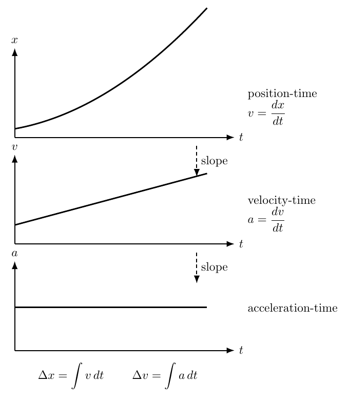
Figure 1. The three standard one-dimensional motion graphs are linked by slopes and signed areas. For constant positive acceleration, position is curved upward, velocity increases linearly, and acceleration is constant.

1 A graph is a representation of a physical quantity

A graph of motion must always be read by identifying both axes. A curve drawn on a position-time graph is not the physical path of the object through space. Instead, the horizontal axis is time and the vertical axis reports the object’s coordinate at each instant.

For one-dimensional motion along an x axis, the three most common graphs are:

x versus t: position as a function of time;
v_x versus t: velocity as a function of time;
a_x versus t: acceleration as a function of time.

The SI units on the vertical axes are respectively meters, meters per second, and meters per second squared.

2 Position-time graphs

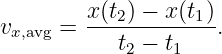
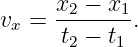
Suppose the position of a particle is x(t). Between times t₁ and t₂, the average velocity is

vx,avg = x(t2) −-x(t1). t2 − t1

(5)

Geometrically, this is the slope of the secant line joining the two points on the position-time graph.

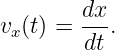
As the interval shrinks to one instant,

dx vx(t) = ---. dt

(6)

Thus the instantaneous velocity is the slope of the tangent to the position-time graph.

This gives several immediate interpretations:

positive slope: v_x > 0;
negative slope: v_x < 0;
horizontal tangent: v_x = 0;
steeper magnitude of slope: larger speed in one dimension.

A horizontal position graph means the object remains at one position during that interval. A graph crossing x = 0 means the particle passes the chosen origin; it does not imply that the particle stops.

3 Piecewise-linear position graphs

A piecewise-linear position graph is especially useful because each straight segment has constant slope and therefore constant velocity on that time interval.

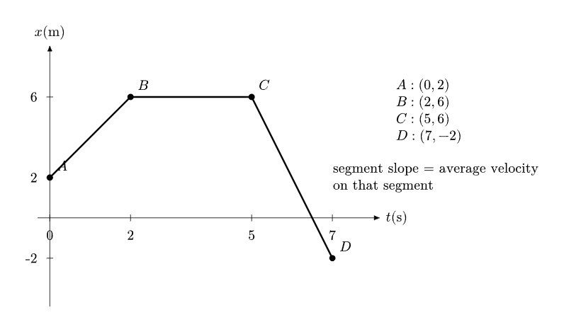
Figure 2. On a piecewise-linear position-time graph, the slope of each segment is the constant velocity on that segment. A horizontal segment represents rest.

For a segment connecting (t₁,x₁) and (t₂,x₂),

x2-−-x1- vx = t − t . 2 1

(7)

A corner in a piecewise-linear idealization means the velocity changes abruptly. Real objects generally require a finite time to change velocity, so such corners are usually simplified models.

4 Velocity-time graphs: slope gives acceleration

If velocity is plotted against time, then

a = dvx-. x dt

(8)

Therefore acceleration is the slope of a velocity-time graph.

The sign of the velocity itself still indicates direction of motion. The sign of the graph’s slope indicates the sign of acceleration. These are distinct pieces of information.

A horizontal velocity-time graph means

ax = 0,

(9)

but the velocity may be positive, negative, or zero.

5 Velocity-time graphs: area gives displacement

From

dx- vx = dt,

(10)

we may write

dx = vxdt.

(11)

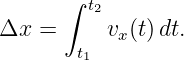
Integrating over a time interval gives

∫ t2 Δx = v (t)dt. t1 x

(12)

Thus the signed area between a velocity-time curve and the time axis is the displacement.

Area above the time axis contributes positively. Area below the time axis contributes negatively.

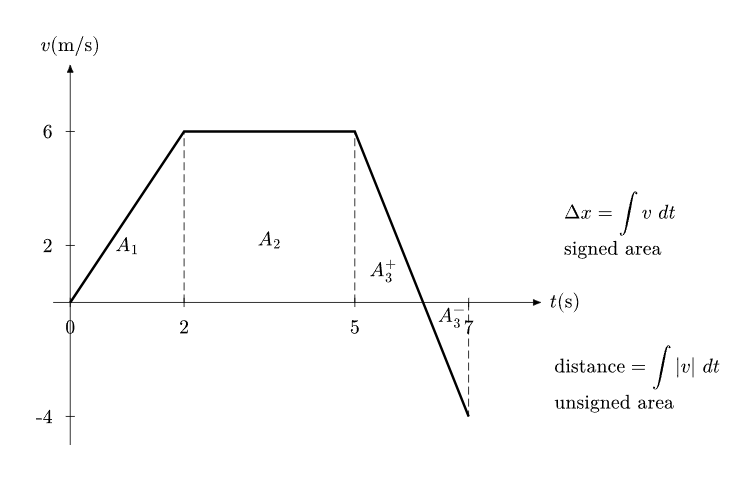
Figure 3. Signed area under a velocity-time graph gives displacement. For distance traveled, areas below the time axis must be counted by magnitude rather than sign.

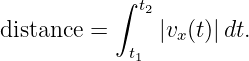
The total distance traveled is instead

∫ t2 distance = |vx(t)|dt. t1

(13)

Therefore distance and displacement are equal only when the velocity does not reverse direction over the interval.

6 Acceleration-time graphs

The acceleration-time graph carries the same slope-area logic one derivative later.

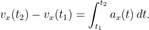
Because

a = dvx-, x dt

(14)

we have

dvx = ax dt.

(15)

Therefore

∫ t 2 vx(t2) − vx(t1) = t ax(t)dt. 1

(16)

The signed area under an acceleration-time graph is the change in velocity, not the velocity itself.

If the initial velocity v_x(t₁) is known, then

∫ t2 vx(t2) = vx(t1) + ax(t)dt. t1

(17)

Similarly, a velocity-time graph determines change in position, but an initial position is required to reconstruct the absolute position.

7 The derivative-integral chain

The three motion graphs form a compact chain:

x(t) −→ v (t) − → a (t) x x

(18)

by differentiation, while integration runs in the reverse direction once the necessary initial values are supplied.

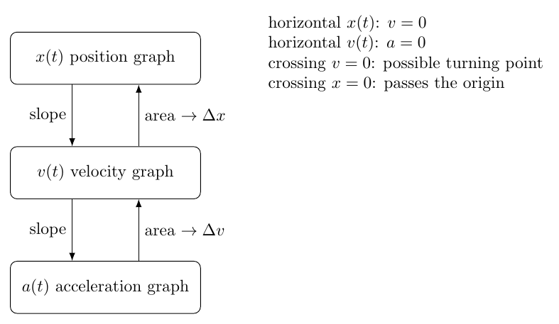
Figure 4. The graph-translation map. Differentiation moves downward from position to velocity to acceleration. Signed areas move upward by giving changes in the next quantity.

This map also helps identify what information is lost when only a derivative graph is known. Acceleration determines how velocity changes, but not the initial velocity. Velocity determines how position changes, but not the initial position.

8 Turning points and zero crossings

Several graph features are frequently confused.

Position crossing zero

If x(t) = 0, the particle is at the chosen origin. Its velocity may be nonzero.

Velocity crossing zero

If v_x(t) = 0, the particle is momentarily at rest in the x direction. If the velocity changes sign across that time, the particle reverses direction and the position graph has a local maximum or minimum.

A zero of velocity is therefore a candidate turning point, but if the velocity touches zero without changing sign, the particle may not reverse.

Acceleration crossing zero

If a_x(t) = 0, the velocity-time graph has zero slope at that instant. The velocity itself need not be zero.

9 Curvature of a position-time graph

Because

d2x ax = dt2-,

(19)

the sign of acceleration is related to the concavity of a smooth position-time graph.

ax > 0,

(20)

the slope dx∕dt increases with time and the position graph is locally concave upward.

ax < 0,

(21)

the slope decreases and the position graph is locally concave downward.

Concavity should not be confused with whether the object is moving in the positive or negative direction. Direction is determined by the sign of slope; concavity is determined by how that slope changes.

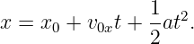
10 Constant acceleration as a graph pattern

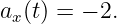
If acceleration is constant,

ax = a,

(22)

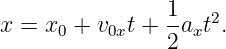
then integrating once gives

vx = v0x + at,

(23)

and integrating again gives

1 x = x0 + v0xt +-at2. 2

(24)

Therefore constant acceleration appears graphically as:

a horizontal line on an acceleration-time graph;
a straight line on a velocity-time graph;
a parabola on a position-time graph.

This visual pattern will be developed further in M01-05.

11 Worked example 1: read a piecewise position graph

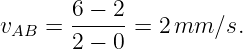
Use Figure 2. The points are

A = (0 ms, 2mm ),

(25)

B = (2 ms, 6mm ),

(26)

C = (5 ms, 6mm ),

(27)

and

D = (7 ms, − 2mm ).

(28)

From A to B,

v = 6 −-2-= 2 mm ∕s. AB 2 − 0

(29)

From B to C,

vBC = 0.

(30)

From C to D,

−-2-−-6 vCD = 7 − 5 = − 4mm ∕s.

(31)

The total displacement is

Δx = − 2 − 2 = − 4 mm.

(32)

Hence the average velocity over the full seven seconds is

− 4 vavg = --- ≈ − 0.571mm ∕s. 7

(33)

The total distance traveled is

4 + 0 + 8 = 12 mm.

(34)

This example shows why distance cannot be found from the overall displacement alone.

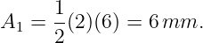
12 Worked example 2: displacement and distance from a velocity graph

Use Figure 3. From 0 to 2 s, the triangular area is

1- A1 = 2 (2)(6) = 6mm.

(35)

From 2 to 5 s, the rectangular area is

A2 = (3)(6) = 18 mm.

(36)

From 5 to 7 s, velocity falls linearly from 6 to −4 m/s. Its slope is

− 4 − 6 a = ------- = − 5 mm ∕s2. 7 − 5

(37)

The velocity reaches zero at

0 = 6 − 5(t − 5),

(38)

t = 6.2ms.

(39)

The positive area from 5 to 6.2 s is

A+ = 1(1.2)(6) = 3.6mm. 3 2

(40)

The negative area from 6.2 to 7 s is

− 1- A 3 = − 2(0.8)(4) = − 1.6 mm.

(41)

Thus the displacement is

Δx = 6 + 18 + 3.6 − 1.6 = 26.0 mm.

(42)

The distance traveled is

6 + 18 + 3.6 + 1.6 = 29.2 mm.

(43)

13 Worked example 3: velocity from an acceleration-time graph

A particle begins with

vx(0) = − 2 mm ∕s.

(44)

Its acceleration is +3 mm∕s² from 0 to 4 s, then −1 mm∕s² from 4 to 7 s.

The first acceleration area gives

Δv1 = (3)(4) = 12mm ∕s.

(45)

Therefore

vx(4 ) = − 2 + 12 = 10 mm ∕s.

(46)

The second interval gives

Δv2 = (− 1 )(3) = − 3 mm ∕s.

(47)

Hence

v (7) = 10 − 3 = 7 mm ∕s. x

(48)

The net area under the acceleration-time graph is 9 mm∕s, which is the net change in velocity.

14 Worked example 4: translate an analytic motion into three graphs

Suppose

2 x(t) = 2 + 3t − t .

(49)

Differentiation gives

vx(t) = 3 − 2t

(50)

and

ax(t) = − 2.

(51)

Therefore the position-time graph is a concave-down parabola, the velocity-time graph is a straight line with slope −2 mm∕s², and the acceleration-time graph is a horizontal line at −2 mm∕s².

The particle reaches a turning point when

vx = 0,

(52)

3 − 2t = 0

(53)

and

t = 1.5ms.

(54)

At that time,

x (1.5) = 2 + 4.5 − 2.25 = 4.25mm.

(55)

The maximum of the position graph and the zero crossing of the velocity graph are therefore the same physical event.

15 Common mistakes

Treating the height of an x-t graph as velocity. Velocity is its slope.
Treating the height of a v-t graph as acceleration. Acceleration is its slope.
Treating area under a velocity graph as distance without accounting for negative velocity.
Assuming x = 0 means the particle is at rest.
Assuming v = 0 means a = 0.
Forgetting that area under an acceleration graph gives change in velocity, not final velocity unless the initial velocity is zero.
Reading a graph as a drawing of the object’s spatial trajectory.

16 Practice problems

M01-04-P01

A position-time graph is a straight line from (0 ms,−2 mm) to (4 ms, 10 mm). Find the velocity.

M01-04-P02

A position-time graph is horizontal at x = 5 mm from t = 2 s to t = 6 s. State the velocity during that interval.

M01-04-P03

A velocity-time graph is constant at v_x = 4 mm∕s for 7 s. Find the displacement.

M01-04-P04

Velocity increases linearly from 0 to 12 mm∕s during 3 s. Find the acceleration and the displacement during the interval.

M01-04-P05

Velocity is +5 mm∕s for 4 s and then −3 mm∕s for 2 s. Find displacement and distance traveled.

M01-04-P06

Acceleration is constant at −2 mm∕s² for 5 s. If the initial velocity is 9 mm∕s, find the final velocity.

M01-04-P07

The area under an acceleration-time graph from t = 1 s to t = 5 s is −6 mm∕s. If v_x(1) = 8 mm∕s, find v_x(5).

M01-04-P08

A particle has

x(t) = 1 − 2t + 4t2.

(56)

Find v_x(t) and a_x(t), and describe the qualitative shapes of the three motion graphs.

M01-04-P09

A velocity-time graph crosses from positive velocity to negative velocity at t = 6 s. What does this imply about the position motion near t = 6 s if the crossing is smooth and the sign changes?

M01-04-P10

A position-time graph is increasing but concave downward. What are the signs of velocity and acceleration?

M01-04-P11

A velocity-time graph is below the time axis but has positive slope. Is the object speeding up or slowing down? Explain using signs.

M01-04-P12

A particle begins at x₀ = −3 mm. The area under its velocity-time graph from 0 to 8 s is +11 mm. Find its final position.

17 Compact answer check

3 mm∕s.
0.
28 mm.
4 mm∕s² and 18 mm.
displacement 14 mm; distance 26 mm.
−1 mm∕s.
2 mm∕s.
v_x = −2 + 8t and a_x = 8; x(t) is concave upward, v_x(t) is a rising straight line, and a_x(t) is a positive horizontal line.
The particle is momentarily at rest and reverses direction; the position graph has a local extremum.
v_x > 0 and a_x < 0.
Slowing down, because v_x < 0 while a_x > 0.
x_f = 8 mm.

18 Connection to the next article

Motion graphs provide the visual structure behind the constant-acceleration formulas. M01-05 develops those formulas systematically from the conditions

ax = constant,

(57)

vx = v0x + axt,

(58)

and

x = x + v t + 1a t2. 0 0x 2 x

(59)

References

[1] PhysicsLibrary, M01-01: Position and Displacement in Mechanics.

[2] PhysicsLibrary, M01-02: Velocity in Mechanics.

[3] PhysicsLibrary, M01-03: Acceleration in Mechanics.

[4] OpenStax / cnxuniphysics, University Physics Volume 1, archived 2016 BCcampus clone, CC BY 4.0.

[5] University of California, Davis, Physics 9A: Classical Mechanics, Physics LibreTexts, CC BY-SA 4.0.

[6] J. R. Taylor, Classical Mechanics, University Science Books, 2005. Used as a scope and notation reference.

"Motion Graphs in Kinematics" is owned by bloftin.
(view preamble)