Minimum-Effort Interception of a Moving Target: Transversality as a Bridge to Optimal
Control
Purpose of this example
CV05 introduced transversality as the endpoint condition that appears when a terminal point is
not fixed, but is constrained to lie on a curve. The phrase “endpoint constrained to a curve” can
sound geometrically abstract. This example gives it an immediate physical interpretation: a vehicle
must intercept a target whose position changes with time.
The target trajectory itself is the terminal constraint curve. The interception point is not known
beforehand. The optimizer is allowed to choose when and where on that curve the interception
occurs. The Euler–Lagrange equation determines the stationary motion in the interior; the
transversality condition determines how that motion must meet the moving terminal
constraint.
The example is deliberately based on the first-order kinematic model
so that the transversality idea is not hidden by higher-order dynamics. The control u is a directly
commanded velocity. Later optimal-control models may replace this by acceleration, thrust,
steering angle, or another physical input.
1 Problem statement: intercept a moving target
A one-dimensional vehicle starts at
A target begins a distance d > 0 ahead and moves away at constant speed V > 0:
The interception time T is not prescribed. At interception, the vehicle must satisfy
Thus the terminal point (T,x(T)) may slide anywhere along the target line in the (t,x)
plane.
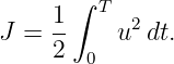
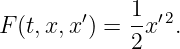
We minimize the quadratic control-effort functional
Using u = x′, this becomes the variational problem
subject to Eqs. (2) and (4), with T free.
The phrase minimum effort here means minimum quadratic control cost. It is not, in general,
literal fuel consumption or mechanical work. The example is intended to expose the variational
endpoint structure as cleanly as possible.[3, 4]
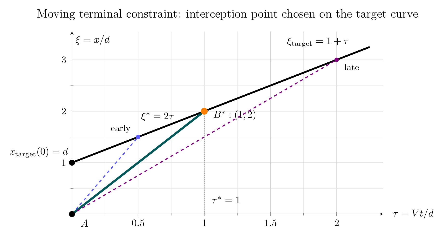
Figure 1. The terminal point is not a prescribed point. It may slide along the moving target
trajectory x = d + V t. For each trial interception time, the stationary interior path is a straight
line. Transversality selects the particular point on the target curve at which the optimum occurs.
2 Why this is a transversality problem
In the generic notation of CV05, the independent variable was called x and the dependent function
was y(x). Here it is more natural to use time t as the independent variable and position x(t) as the
dependent function. The translation is therefore
The terminal point is
Because T is free, the endpoint may move horizontally in the (t,x) plane. Because the vehicle must
remain on the target trajectory at interception, the vertical terminal displacement is not
independent of that horizontal motion.
For the target curve
an allowed endpoint displacement obeys the linearized constraint
Equation (10) says that the endpoint may move, but only tangent to the target curve. This is
exactly the endpoint geometry for which CV05 derived a transversality condition.
3 Deriving the moving-endpoint variation for this problem
Because the movement of the endpoint is central to this example, we derive the terminal variation
rather than simply quoting the final formula.
Introduce a one-parameter family of nearby curves
and allow the terminal time to vary as
The perturbed functional is
where, for the present problem,
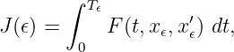
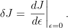
The first variation is
The upper integration limit depends on 𝜖, so the Leibniz rule gives
The final term has a simple geometric interpretation. Moving the upper limit from T to T + δT
adds, to first order, a thin strip with width δT and height F(T), hence the contribution
F(T)δT.
Integrate the second term in Eq. (16) by parts:
| ∫
0T F
x′η′dt | = ![[Fx′η]](https://images.physicslibrary.org/cache/objects/1324/make4ht/MinimumEffortInterceptionOfAMovingTarget16x.png) 0T −∫
0T 0T −∫
0T  Fx′η dt. Fx′η dt. | (17) |
Therefore
The initial point is fixed, so
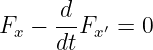
For a stationary curve, the interior Euler–Lagrange equation
eliminates the integral term. The terminal contribution becomes
4 The distinction between η(T) and the actual endpoint motion
Equation (21) contains η(T), but when the terminal time moves, η(T) is not the same quantity as
the actual vertical endpoint displacement δxT .
The perturbed endpoint position is
Substituting Eq. (11),
Taylor-expand to first order in 𝜖:
| x(T + 𝜖δT) | = x(T) + 𝜖x′(T)δT + O(𝜖2), | (24)
|
| 𝜖η(T + 𝜖δT) | = 𝜖η(T) + O(𝜖2). | (25) |
Hence
The actual first-order terminal displacement is therefore
Equivalently,
This is the same moving-endpoint linearization developed in CV05. One term comes from
deforming the curve at fixed t = T; the other comes from sliding the endpoint along the original
curve.
Substitute Eq. (28) into Eq. (21):
| δJT | = Fx′ + FδT + FδT | (29)
|
| = Fx′δxT + 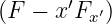 δT. δT. | (30) |
Thus the universal terminal boundary form in the (t,x) plane is
5 Apply the target-curve constraint
The endpoint must remain on the moving target line. Therefore Eq. (10) gives
Substitute into Eq. (31):
| δJT | = Fx′V δT + 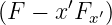 δT δT | (33)
|
| = ![′ ′
[F + (V − x)Fx ]](https://images.physicslibrary.org/cache/objects/1324/make4ht/MinimumEffortInterceptionOfAMovingTarget32x.png) δT. δT. | (34) |
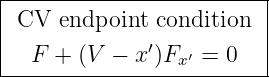
The interception point is free to move along the target trajectory, so δT is arbitrary. Stationarity
therefore requires
This is the transversality condition for this moving-target problem.
The key contrast with a natural boundary condition is worth emphasizing. A natural boundary
condition appears when a terminal coordinate is freely variable by itself. Here the terminal
variations are linked:
The endpoint has one degree of freedom, but that freedom lies tangent to the target curve.
Transversality is the stationarity condition associated with that constrained endpoint
motion.
6 Euler–Lagrange equation in the interior
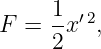
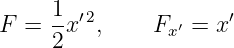
For
we have
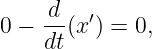
The Euler–Lagrange equation is therefore
or
Integrating twice,
The fixed initial condition x(0) = 0 gives C0 = 0, so
Thus the stationary interior trajectory uses a constant velocity command. The remaining question
is: which constant velocity, and which interception point on the target curve? That is precisely
what the terminal constraint and transversality condition determine.
7 Use transversality to determine the optimal control
Substitute
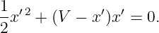
into Eq. (35):
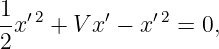
Expand:
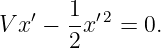
so
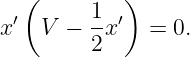
Factor:
The root x′ = 0 cannot intercept a target that begins at d > 0. The nontrivial stationary solution
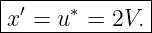
is therefore
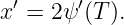
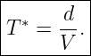
The terminal constraint now determines T:
Hence
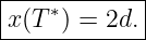
The interception position is
The target travels a distance d during the optimal interception interval, so it moves from x = d
to x = 2d. The vehicle travels twice that distance from the origin, at twice the target
speed.
8 What does the solution mean physically?
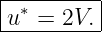
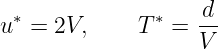
The result
has a useful physical interpretation.
If the vehicle tries to intercept too early, the target has not moved very far, but the vehicle must
cover the initial gap d in a very short time. The required command u is large, and the quadratic
penalty u2 makes that expensive.
If the vehicle waits too long, the required excess speed above the target speed is smaller, but the
target continues to move away and the control must be applied over a longer interval. The
accumulated cost again becomes large.
The optimum balances these two effects. At T = d∕V , the target has moved exactly
one initial-gap distance d. The vehicle has traveled 2d, and the relative closing speed
is
Thus the time needed to close the original gap is
The transversality condition has therefore selected both a terminal point and a control level with a
simple physical meaning.
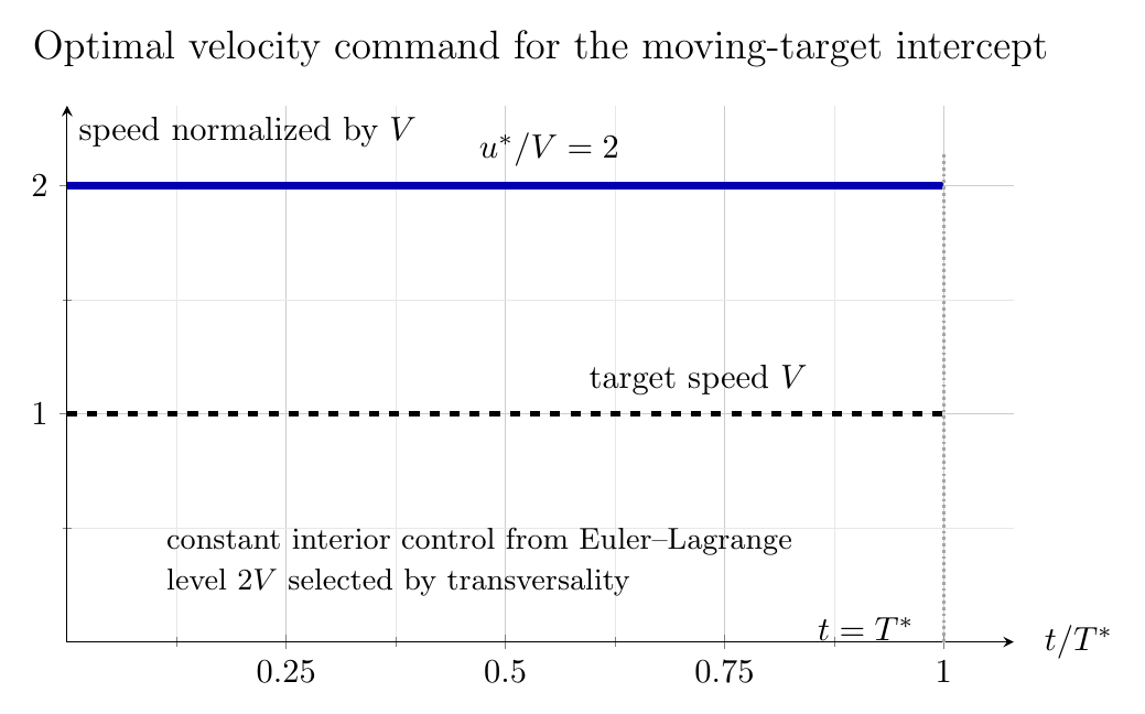
Figure 2. The stationary interior solution has constant control because x′′ = 0. Transversality
selects the particular level u∗ = 2V . The target moves at speed V , so the optimal vehicle
command is twice the target speed.
9 An independent check: optimize directly over interception time
There is a useful way to verify the transversality result without using the moving-endpoint
formula.
Suppose temporarily that a trial interception time T has been chosen. The terminal point is then
fixed at
For this fixed T, the Euler–Lagrange equation gives a constant-speed path from 0 to
d + V T:
The corresponding cost is
| J(T) | =  uT 2T uT 2T | (57)
|
| =   2T 2T | (58)
|
| =  + dV + + dV +  . . | (59) |
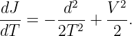
Differentiate:
Stationarity gives
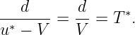
Because T > 0, d > 0, and V > 0,
exactly as obtained from transversality.
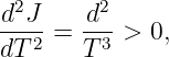
Moreover,
so this stationary value is a strict minimum with respect to the interception time.
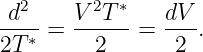
At the optimum, the two T-dependent contributions in Eq. (59) are equal:
This equality gives another interpretation of the optimum: the cost associated with closing
the initial spatial gap and the cost associated with the target’s continued motion are
balanced.
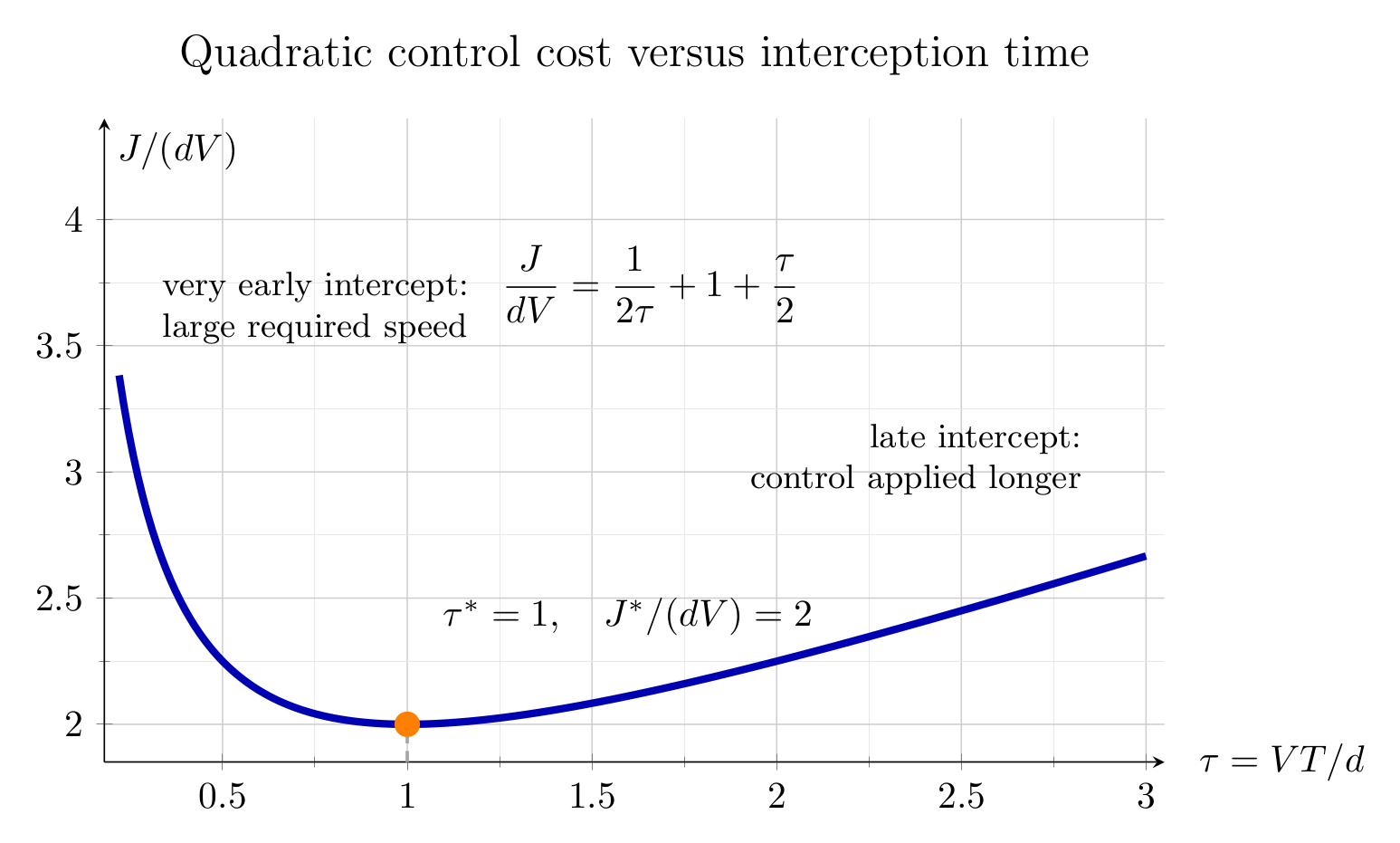
Figure 3. Normalized cost versus normalized interception time. Very early interception is
expensive because the required speed is large; very late interception is expensive because the
control is maintained while the target continues to move away. The minimum occurs at V T∕d = 1.
10 Minimum cost
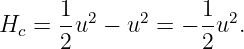
Substitute Eqs. (48) and (50) into the objective:
| J∗ | =  ∫
0d∕V (2V )2 dt ∫
0d∕V (2V )2 dt | (65)
|
| =  (4V 2) (4V 2) . . | (66) |
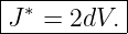
Therefore
The units are those of the mathematical quadratic control cost. Since u is a velocity command
here,
This should not be interpreted automatically as mechanical energy.
11 Numerical example
Take
The transversality solution gives
and
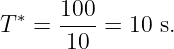
The target begins at 100 m and moves another 100 m during those ten seconds, so the
interception occurs at
The minimum quadratic control cost is
The vehicle’s relative closing speed is
so closing the initial 100 m gap takes exactly 10 s.
12 Geometric meaning of transversality
Define the momentum-like endpoint coefficient
and the Hamiltonian-like quantity
Then the terminal boundary form, Eq. (31), becomes
The terminal target curve has tangent displacement
Equation (77) can therefore be written as the dot product
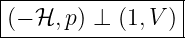
Stationarity requires this dot product to vanish for every allowed tangent motion. Hence
The boundary covector is normal to the terminal constraint curve. This is the geometric content of
the word transversality.
For the present integrand,
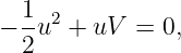
Thus Eq. (80) gives
which again yields the nontrivial solution u = 2V .
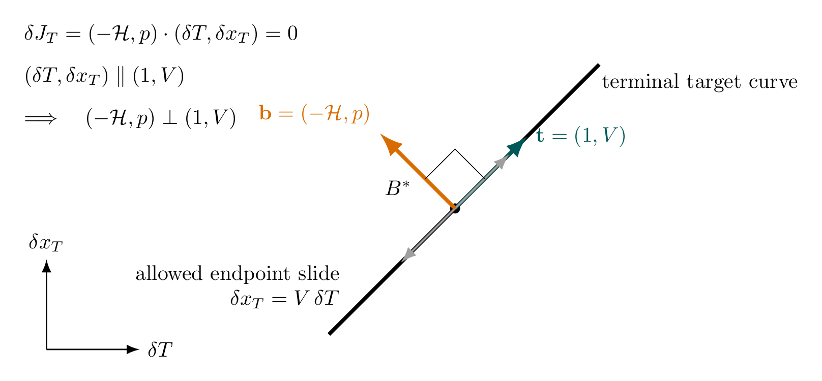
Figure 4. At the selected terminal point, allowed endpoint motion is tangent to the target curve.
The variational boundary covector (−ℋ,p) must annihilate that tangent motion and is therefore
normal to the target curve. This orthogonality in endpoint-variation space is the geometric
meaning of transversality.
13 The same result in optimal-control language
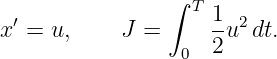
Now rewrite the problem exactly as an elementary optimal-control problem:
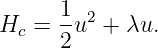
Use the minimization-convention control hamiltonian
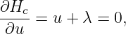
Stationarity with respect to u gives
so
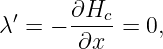
The costate equation is
so the costate is constant, and therefore the optimal control is constant. This is the same
conclusion obtained from the Euler–Lagrange equation x′′ = 0.
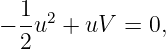
The terminal condition is not a fixed terminal state. It is the terminal manifold
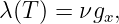
Introduce a terminal multiplier ν. The standard transversality conditions for this equality
constraint, with no terminal cost, are
and
For Eq. (88),
Therefore
and
From Eq. (86), ν = λ = −u. On the stationary control,
Thus the terminal condition becomes
and again
The same terminal geometry has therefore appeared in three equivalent forms:
and
The first is classical calculus of variations, the second is its geometric boundary interpretation, and
the third is the terminal transversality language of optimal control.[3, 4]
14 Natural boundary condition versus transversality
CV05E2 considered a free terminal state coordinate. This article considers a terminal point
constrained to a curve. The distinction can be summarized as follows.
|
|
|
Endpoint type | Allowed variation | Boundary consequence |
|
|
|
Fixed terminal
coordinate | Variation of that coordinate
is zero | No new boundary equation
from that coordinate |
|
|
|
Free terminal
coordinate | Variation is arbitrary and
independent | Its conjugate boundary
coefficient must vanish |
|
|
|
Endpoint constrained
to a curve | Endpoint
variations are nonzero but
linked by the curve tangent | A linear combination
of boundary coefficients must
vanish: transversality |
|
|
|
In the present example,
is the crucial relation. Neither δxT nor δT is forced to zero, but they cannot vary independently.
That is why the terminal condition is not simply Fx′ = 0 or F − x′Fx′ = 0. Instead the two
coefficients combine according to the tangent direction of the target curve.
15 Generalization to a nonlinear moving target
Suppose the target trajectory is a smooth nonlinear function
Then an allowed terminal displacement satisfies
The transversality condition becomes
For F =  x′2, the nontrivial terminal condition reduces to
The interior Euler–Lagrange equation still requires x′ to be constant in this simple
single-integrator model, so the interception time must satisfy both
and
For a nonlinear target path, these equations may need to be solved numerically. This is already
very close in spirit to practical trajectory optimization.
16 What should be carried forward into optimal control?
This example provides several ideas that recur in more advanced trajectory optimization:
- The terminal state need not be a prescribed point. It may lie on a terminal curve,
surface, or higher-dimensional manifold.
- The Euler–Lagrange equations govern the stationary trajectory in the interior, but
they do not by themselves determine which terminal point on the constraint should be
selected.
- Allowed endpoint variations are tangent to the terminal constraint.
- The variational boundary covector must annihilate every allowed tangent displacement;
geometrically, it is normal to the terminal constraint.
- In optimal control, the same normality condition is expressed through terminal costates
and multipliers.
- A transversality condition is a necessary stationarity condition. It does not by itself
prove that the stationary trajectory is a minimum.
For the moving-target problem, the conceptual chain is
Summary
A kinematic vehicle obeying
must intercept a target
while minimizing
The final time is free, and the final point must lie on the target trajectory. The moving-endpoint
first variation produces
Because the target curve imposes
stationarity requires
For
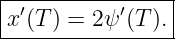
Euler–Lagrange gives constant x′, while transversality selects
The terminal constraint then gives
The example shows concretely what it means for an endpoint to be “constrained to a curve.” The
terminal point may move, but only tangent to the target trajectory. Transversality supplies the
boundary equation associated with that constrained motion, and the same structure becomes a
terminal-manifold condition in optimal control.
References
References
[1] I. M. Gelfand and S. V. Fomin, Calculus of Variations, Prentice-Hall, 1963; reprinted
by Dover Publications.
[2] B. van Brunt, The Calculus of Variations, Springer, 2004.
[3] D. Liberzon, Calculus of Variations and Optimal Control Theory: A Concise
Introduction, Princeton University Press, 2012.
[4] D. E. Kirk, Optimal Control Theory: An Introduction, Prentice-Hall, 1970.
![[parent]](https://images.physicslibrary.org/images/uparrow.png)




![∫
1- T 2
J [u ] = 2 u (t)dt.
0](https://images.physicslibrary.org/cache/objects/1324/make4ht/MinimumEffortInterceptionOfAMovingTarget4x.png)
![|--------∫--T---------|
J [x ] = 1 x′2(t)dt |
| 2 0 |
----------------------](https://images.physicslibrary.org/cache/objects/1324/make4ht/MinimumEffortInterceptionOfAMovingTarget5x.png)







![∫ ( )
T -d T
δJ = Fx − dtFx ′ ηdt + [Fx ′η ]0 + F (T)δT.
0](https://images.physicslibrary.org/cache/objects/1324/make4ht/MinimumEffortInterceptionOfAMovingTarget18x.png)




![x 𝜖(T𝜖) = x(T ) + 𝜖[η (T ) + x′(T )δT ] + O (𝜖2).](https://images.physicslibrary.org/cache/objects/1324/make4ht/MinimumEffortInterceptionOfAMovingTarget24x.png)
















![2
[J ] = length--.
time](https://images.physicslibrary.org/cache/objects/1324/make4ht/MinimumEffortInterceptionOfAMovingTarget69x.png)