From Goddard’s Unsolved Variational Rocket Problem to Saturn IGM: Calculus of Variations in
Rocket Development
The calculus of variations entered modern rocketry before liquid-fueled rockets had even
flown.
In 1916 Robert H. Goddard wrote to the Smithsonian Institution that his theoretical rocket
problem had forced him to use an approximation in order to avoid what he called “a new and
unsolved problem in the Calculus of Variations.”
Three years later his A Method of Reaching Extreme Altitudes made the issue explicit.
Goddard wanted to determine a rocket ascent for which the initial mass required to deliver a
specified final mass to a specified altitude would be a minimum.
That is an optimization problem over an entire trajectory, not merely an algebra problem at one
instant.
By the Apollo era, the same broad mathematical idea had become practical engineering.
The Saturn launch vehicle did not solve the full nonlinear calculus-of-variations boundary-value
problem aboard the vehicle.
Instead, Marshall Space Flight Center engineers used variational optimization to identify a simple
near-optimal steering structure, then built an iterative digital guidance algorithm around that
structure.
The result was the Saturn Iterative Guidance Mode, or IGM.
This article follows that history:
- Goddard’s early minimum-mass ascent problem,
- the later mathematical development of optimum rocket trajectories,
- the V-2, Redstone, Jupiter, and Pershing guidance lineage,
- the Army ballistic Missile Agency transition to NASA Marshall,
- the variational origin of linear tangent steering,
- the way Saturn IGM converted an optimization result into an onboard guidance law.
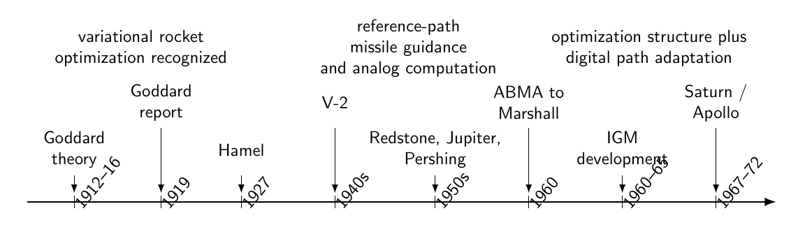
Figure 1. A compressed historical timeline. Goddard recognized the variational structure of
rocket optimization before practical liquid-fuel rocketry existed. Army missile guidance later
emphasized reference-trajectory correction, while the Saturn era combined optimization
theory with digital onboard computation.
1 A necessary historical distinction
There was not one continuous algorithm passed unchanged from Goddard to Apollo.
Several different lines of development converged.
The three lines can be summarized without treating them as one continuous algorithm:
- Mathematical line: rocket performance led to trajectory optimization and then to
calculus-of-variations formulations.
- Missile-guidance line: V-2 experience led into Redstone, Jupiter, and Pershing, with
analog computation and reference-trajectory correction.
- Computational line: ground-based optimization was gradually joined by digital
onboard computation and path-adaptive guidance.
The historical importance of IGM is that these lines finally met.
2 Goddard’s question was already variational
Goddard’s 1919 report begins with a performance question.
Suppose a rocket loses mass continuously while climbing vertically.
A final payload mass is to remain when the rocket reaches a required altitude.
What initial mass is necessary?
Goddard did not merely ask for the motion produced by a prescribed rocket.
He asked which motion minimizes the required mass.
He wrote the vertical speed as an unknown function of altitude:
where
is altitude.
The expelled mass then depends on the entire function
The goal is therefore schematically
That is the structure of a calculus-of-variations problem.
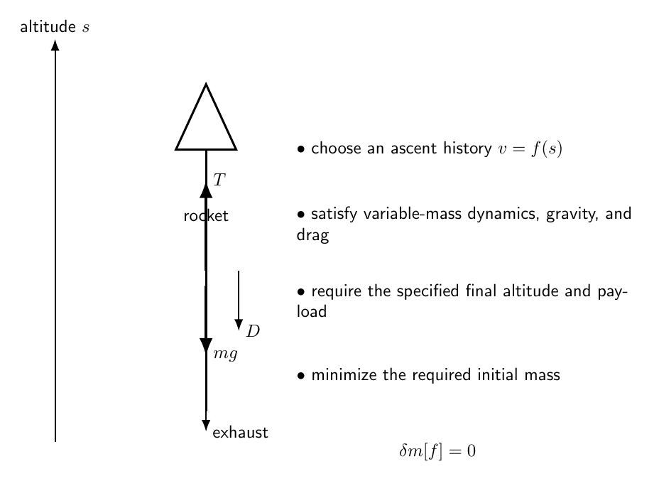
Figure 2. Goddard’s vertical rocket problem. Gravity and atmospheric resistance oppose
ascent while propellant mass is expelled. The unknown is not one number but an ascent
history, which is why minimization naturally becomes a variational problem.
3 Why ordinary differential equations were not enough
If the thrust or mass-loss history were already known, the equations of motion could be
integrated.
Optimization changes the nature of the problem.
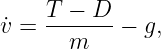
The trajectory must satisfy dynamics such as
and
while a performance quantity is extremized.
Here:
 is altitude,
 is vertical speed,
 is rocket mass,
 is thrust,
 is drag,
 is effective exhaust velocity.
A modern Goddard-type problem can be stated as
or, in a form closer to Goddard’s original concern,
subject to prescribed final conditions.
The optimization therefore includes a function such as
or an equivalent burning history.
4 Goddard’s unsolved calculus-of-variations problem
In the published report Goddard explained that the minimum requires an unknown velocity
function
for which
He then stated that determining this function by the rigorous procedure led to a new and unsolved
calculus-of-variations problem.
Instead of stopping, he constructed an approximate procedure.
He divided the ascent into altitude intervals, treated important quantities approximately within
each interval, and searched for the minimum mass required in each segment.
The historical lesson is important:
- Rocket optimization appeared before the mathematical and computational machinery
needed to solve the realistic problem cleanly.
5 Goddard was asking an optimal-control question before optimal control existed
The modern language of states and controls came later.
Retrospectively, Goddard’s problem contains all of the basic elements:
- dynamical state variables,
- a controllable burning history,
- variable mass,
- gravity,
- drag,
- endpoint requirements,
- an integral or terminal performance criterion.
This is the same general structure later formalized by:
- the classical calculus of variations,
- the Mayer, Lagrange, and Bolza problem formulations,
- the Pontryagin maximum principle,
- modern optimal control.
It is therefore reasonable to call the later vertical ascent optimization problem the Goddard
problem, but the modern textbook form should not be confused with every detail of Goddard’s
original 1919 approximation.
6 Hamel and the interwar mathematical continuation
The problem did not disappear.
Georg Hamel returned to Goddard’s rocket optimization problem in 1927 and treated the optimum
burning program explicitly with calculus-of-variations methods.
Later historical reviews of optimal flight mechanics identify Goddard and Hamel as early examples
of applying variational ideas to rocket-powered flight.
During the following decades, increasingly general formulations were developed for:
- optimum climb,
- minimum fuel,
- maximum altitude,
- maximum range,
- constrained flight paths.
By the 1950s and early 1960s, the mathematical literature on optimum rocket trajectories had
become much richer.
Later reviews list work by Tsien and Evans, Miele and Cavoti, Leitmann, Garfinkel, and others as
part of the continuing development of the Goddard problem.
7 The wartime and missile-guidance line developed differently
The practical guidance systems of early ballistic missiles were not simply onboard
calculus-of-variations solvers.
A missile had to:
- sense attitude and acceleration,
- reject disturbances,
- follow a useful trajectory,
- shut down propulsion at the correct condition,
- operate with the computers available at the time.
The available hardware strongly shaped the guidance philosophy.
8 V-2 to Redstone, Jupiter, and Pershing
Clyde D. Baker’s 1965 historical summary of Saturn guidance described an important
lineage.
Beginning with the V-2 and continuing through the Army’s Redstone, Jupiter, and Pershing
missiles, the delta-minimum concept was used successfully.
Its basic philosophy was:
- determine a nominal geometrical trajectory before flight,
- measure how the actual vehicle differs from that reference,
- command corrections that drive the vehicle back toward the reference trajectory.
The nominal trajectory was determined before flight.
Guidance corrections attempted to reduce deviations from it.
Analog computation was well suited to this type of implementation.
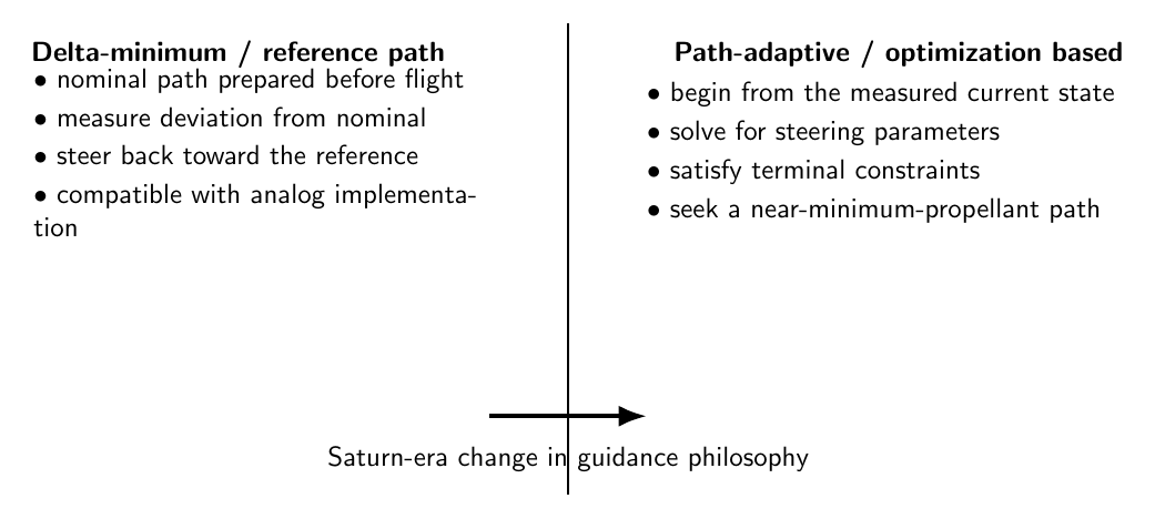
Figure 3. Delta-minimum guidance and variational guidance answer different questions.
Delta-minimum tries to recover a precomputed reference path. Variational guidance asks what
steering history best satisfies a performance objective and terminal constraints from the state
that actually exists.
9 Why delta-minimum worked for missiles
For a ballistic missile:
- the mission geometry was highly repeatable,
- the desired path could be designed before launch,
- onboard analog computing resources were limited,
- returning toward a known reference trajectory was a practical strategy.
This did not mean optimization was irrelevant.
Optimum trajectories could still be designed on the ground.
But the onboard guidance system did not have to solve a new optimum trajectory during
flight.
10 The U.S. Army rocket-development bridge
After World War II, the German rocket team and U.S. Army missile organizations developed a
sequence of increasingly capable vehicles.
The Redstone became the first operational U.S. large ballistic missile.
The Jupiter program extended Army ballistic-missile experience.
Pershing continued the tactical ballistic-missile line.
Jupiter-C and Juno connected that missile technology to early U.S. space launch.
The same broad technical community in Huntsville then became central to Saturn.
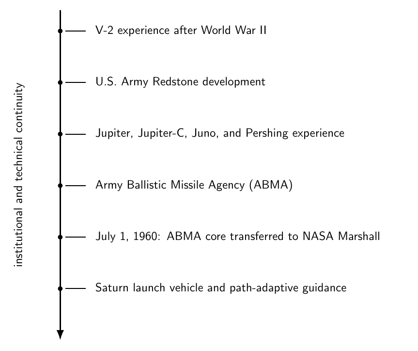
Figure 4. The institutional and technical bridge from Army rocketry to Saturn. The Army
Ballistic Missile Agency concentrated experience in propulsion, inertial guidance,
computation, testing, and flight mechanics. Its core transferred to NASA Marshall in 1960.
11 The Army Ballistic Missile Agency
The Army Ballistic Missile Agency, ABMA, was created in 1956 around the Redstone development
organization.
Its work included:
- Redstone,
- Jupiter,
- Jupiter-C,
- early Saturn concepts,
- inertial guidance and control,
- flight computation and simulation.
On July 1, 1960, the technical and administrative core of ABMA transferred to NASA and became
the George C. Marshall Space Flight Center.
That institutional continuity matters.
Saturn guidance did not begin in isolation.
It grew from engineers already experienced with V-2-derived and Army missile technology, but who
now faced a substantially different space-launch problem.
12 Why Saturn required a different guidance philosophy
Baker identified two changes around 1960.
First, new optimization methods made payload maximization and minimum-propellant trajectory
design increasingly practical.
Second, digital computers were replacing analog computers as onboard hardware.
Saturn also demanded greater mission flexibility.
A space launch vehicle might have to accommodate:
- engine-performance dispersions,
- staging variations,
- engine-out conditions,
- different orbital targets,
- translunar injection conditions.
For this environment, forcing every disturbed flight back toward one nominal geometrical
trajectory was unnecessarily restrictive.
A better guidance question was:
- Given the vehicle’s measured state now, what thrust direction should be commanded
so that the required terminal conditions are still achieved with nearly minimum
propellant?
That is much closer to an optimal-control question.
13 The full optimum Saturn problem was still too difficult onboard
A realistic Saturn optimization model would include:
- a rotating Earth,
- spheroidal gravity,
- multiple stages,
- changing thrust and mass,
- coast intervals,
- three-dimensional motion,
- terminal position and velocity requirements.
In principle, calculus-of-variations methods can formulate this problem.
But Baker explicitly noted that the full optimum-thrust-direction calculation required
computational resources far beyond the onboard computer capability of the time.
The engineering solution was therefore not to abandon optimization.
It was to simplify the variational problem until its structure could be carried onboard.
14 The simplified variational model
Consider vacuum powered flight over a flat Earth with constant gravity.
Use two position coordinates:
downrange and
vertical.
The simplified dynamics are
The thrust magnitude history
is treated as known from the vehicle model.
The control is the thrust direction
15 A variational derivation of the steering structure
Introduce multipliers
for the position and velocity equations.
An augmented integrand can be written schematically as
| ℒ | = px(vx −ẋ) + py(vy −ẏ) | (22)
|
| + qx(a cos 𝜃 −vx) | (23)
|
| + qy(a sin 𝜃 − g −vy). | (24) |
Stationarity with respect to the states gives the adjoint structure
and
Therefore the velocity multipliers are affine functions of time.
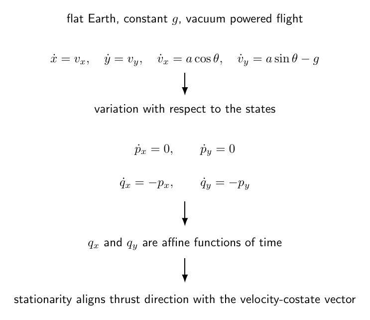
Figure 5. The crucial mathematical simplification behind linear tangent steering. In the
flat-Earth constant-gravity variational model, position costates are constant and velocity
costates are affine in time. Stationarity aligns thrust with the velocity-costate vector.
16 Why a tangent becomes linear
Suppose the final downrange position is free.
The corresponding transversality condition gives
Then
is constant, while
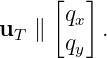
Stationarity with respect to thrust direction gives
Hence
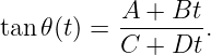
This is the linear tangent steering law.
The angle itself is not linear.
Its tangent is.
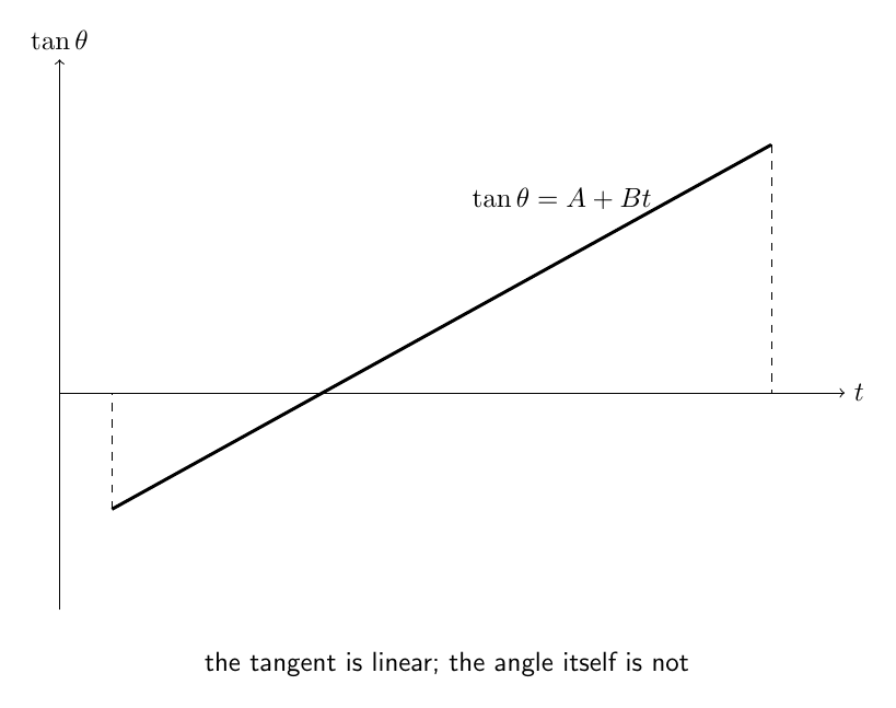
Figure 6. Linear tangent steering. The variational solution gives a thrust-direction law of the
form  under the simplified model and appropriate terminal freedom. Saturn
guidance used this optimal-law structure rather than solving the full variational
boundary-value problem onboard.
17 If both endpoint coordinates are constrained
If the downrange terminal coordinate is also constrained, then generally
Both
and
are affine in time.
The steering law then has the more general form
This later appears naturally in generalized linear-tangent and powered-explicit guidance
formulations.
The simpler Saturn IGM structure can be understood as exploiting a special but highly useful
variational result.
18 From the optimal law to IGM
The key engineering insight was:
- do not integrate a full calculus-of-variations boundary-value problem onboard; use the
shape of its optimal steering law and solve only for the coefficients needed to hit the
target.
The Iterative Guidance Mode repeatedly:
- read the current navigation state,
- estimate time-to-go,
- evaluate stage performance integrals,
- solve for steering-law parameters,
- predict terminal position and velocity,
- update the steering command,
- repeat.
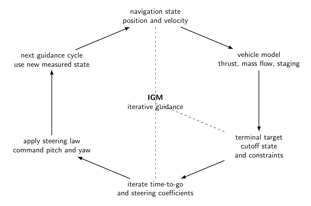
Figure 7. Conceptual IGM loop. The variational calculation supplies the steering-law form.
The onboard digital computer repeatedly updates the law’s coefficients from the measured
state, stage performance, and desired terminal conditions.
19 Why it was called iterative
The vehicle did not receive one fixed steering program and blindly follow it.
IGM continually recalculated quantities such as:
- time remaining to cutoff,
- steering coefficients,
- stage integrals,
- terminal-state predictions.
Each cycle used the current measured state.
This made IGM path adaptive.
A disturbed Saturn did not have to return to exactly the same geometric path that an undisturbed
Saturn would have flown.
It could instead fly a new near-optimal path from its current state to the desired terminal
conditions.
20 IGM was variational in origin, not a full variational solver onboard
This distinction resolves an apparent contradiction in historical descriptions.
Some descriptions say IGM was based on calculus of variations.
Others emphasize that IGM itself did not numerically solve a full calculus-of-variations problem
during flight.
Both statements can be correct.
The full realistic optimum problem was too computationally demanding for the Saturn onboard
computer.
The simplified variational problem supplied the steering-law structure.
IGM then solved an iterative guidance problem within that structure.
The relationship is better read as a sequence of engineering steps:
- calculus of variations supplies the structure of an optimal steering law,
- that structure is simplified into a form suitable for flight computation,
- the onboard guidance system repeatedly solves for the coefficients needed to satisfy the
terminal conditions.
21 The Marshall guidance team
Baker’s 1965 account credited the Saturn iterative-guidance development primarily to Helmut J.
Horn and his associates in the Dynamics Analysis and Flight Mechanics organization at
Marshall.
Later accounts also identify important work by:
- Daniel T. Martin,
- Isaac E. Smith,
- Judson J. Hart,
- Clyde D. Baker,
- later Roland Jaggers in the evolution toward Linear Tangent Guidance.
This was a team development rather than the work of one isolated mathematician.
22 The Army-to-NASA continuity
The organizational transition from ABMA to Marshall preserved deep practical experience in:
- inertial navigation,
- missile control,
- analog simulation,
- flight testing,
- trajectory design.
What changed was the mission.
Army ballistic missiles had emphasized reliable delivery along a mission-specific trajectory.
Saturn had to maximize payload and meet orbital or translunar terminal conditions despite
dispersions.
The combination of:
- Army missile experience,
- variational trajectory theory,
- digital computers
made path-adaptive guidance practical.
23 Saturn V and Apollo
IGM belonged to the Saturn launch vehicle guidance system.
It should not be confused with the guidance equations executed by the Apollo spacecraft computer
after separation.
Nevertheless, during an Apollo launch, Saturn IGM was the launch-vehicle guidance
method responsible for steering the upper stages toward required orbital or translunar
conditions.
Thus the phrase “Apollo IGM” is useful informally only if one remembers that IGM was a Saturn
function within the Apollo launch stack.
24 A dramatic test: AS-502
The value of path-adaptive guidance was demonstrated by flight anomalies.
During Saturn V flight AS-502, the Apollo 6 mission, two S-II stage engines were lost during
powered flight.
NASA’s later guidance-system review reported that IGM still brought the vehicle close to the
required altitude constraint even though the original implementation had been designed around a
less severe engine-out case.
This is precisely the kind of situation in which a path-adaptive law is more useful than simply
forcing the vehicle back toward one nominal path.
25 The first-stage limitation
Saturn did not apply the same optimum vacuum guidance law from liftoff.
During the high-dynamic-pressure part of first-stage flight:
- aerodynamic loads mattered strongly,
- angle of attack had to remain small,
- structural bending and heating imposed constraints.
A programmed tilt trajectory was therefore used during the early atmospheric phase.
Closed-loop iterative guidance became most natural after the vehicle had left the severe
atmospheric-load region.
This also illustrates a general principle:
- An optimal law derived for one model is not automatically optimal when the neglected
physics becomes important.
26 What calculus of variations actually contributed
The calculus of variations did not contribute just one formula.
It contributed a way to think.
The change in viewpoint can be stated as two questions:
- Forward simulation: What trajectory will this prescribed steering program produce?
- Trajectory optimization: What steering program extremizes payload, fuel, time,
altitude, or another mission objective while satisfying the equations of motion and
terminal constraints?
That reversal is the conceptual foundation of trajectory optimization.
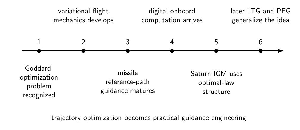
Figure 8. The historical role of calculus of variations in rocketry. It began as an analysis
problem that Goddard could only approximate, matured into trajectory-optimization theory,
and finally supplied simple optimal steering structures that could be embedded in practical
digital guidance.
27 The most important historical transition
The deepest transition was not merely a change from analog to digital computation.
It was a change in guidance philosophy:
- earlier systems emphasized correction back toward a reference path,
- Saturn-era guidance increasingly emphasized finding a feasible near-optimal path from
the measured state to the required target conditions.
Digital computation made that transition practical onboard.
Calculus of variations supplied the mathematical structure.
28 From IGM to later guidance
The story did not stop with Saturn.
The same line of reasoning evolved into:
- generalized Linear Tangent Guidance,
- Apollo-era guidance-theory studies,
- Shuttle Powered Explicit Guidance,
- later launch-vehicle explicit guidance methods.
Later guidance systems changed models, constraints, and numerical methods.
But the historical pattern remained recognizable:
- formulate an optimum trajectory problem,
- derive structure from variational or optimal-control theory,
- simplify that structure into a form suitable for onboard computation,
- update the solution using the measured state.
29 Goddard and IGM side by side
The historical symmetry is striking.
Goddard faced a realistic optimization problem whose rigorous variational solution was beyond the
practical mathematics available to him.
He therefore built an approximate method that preserved enough of the physics to answer the
engineering question.
Half a century later, Saturn engineers faced a realistic optimization problem whose
full variational solution was beyond the practical onboard computation available to
them.
They also simplified the problem while preserving the essential optimal structure.
The difference was that the simplified law could now be recomputed repeatedly during
flight.
30 A compact mathematical comparison
The two problems can be compared directly:
- Goddard: choose an ascent history that minimizes the required initial mass or expelled
propellant.
- Saturn vacuum guidance: choose a thrust-direction history that reaches the
terminal conditions with near-minimum propellant.
Both are trajectory optimization problems.
Both require choosing a function, not merely one scalar.
Both naturally lead to variational reasoning.
31 Historical cautions
Several oversimplifications should be avoided.
- Goddard did not derive Saturn IGM.
- The V-2, Redstone, Jupiter, and Pershing did not use Saturn IGM.
- Army delta-minimum guidance was not the same as calculus-of-variations optimal
guidance.
- Saturn IGM did not numerically solve the full rotating-Earth calculus-of-variations
problem onboard.
- Modern optimal-control versions of the Goddard problem contain later mathematical
developments and should not be treated as identical to Goddard’s original 1919
calculation.
- IGM was Saturn launch-vehicle guidance used during Apollo missions, not an Apollo
spacecraft guidance mode.
These distinctions make the historical connection stronger rather than weaker.
They show how an abstract optimization idea gradually became an engineering method.
32 Study questions
- Why does minimizing initial rocket mass require choosing an entire function rather
than one number?
- In modern notation, identify possible state and control variables in Goddard’s
vertical-ascent problem.
- Why did Goddard resort to an approximate interval method?
- What is the conceptual difference between delta-minimum guidance and path-adaptive
guidance?
- Why were analog computers naturally associated with early reference-trajectory missile
guidance?
- What institutional connection linked Army ballistic-missile development to NASA
Marshall?
- Why was the full optimum Saturn guidance problem unsuitable for direct onboard
variational solution?
- Starting from the simplified flat-Earth equations, derive
- Show that free final downrange position implies a constant horizontal velocity
costate.
- Derive
- Explain why linear tangent steering is an optimal-law structure rather than a complete
guidance system.
- Explain why IGM is both variational in origin and not a full onboard calculus-of-variations
solver.
- Why does engine-out capability favor path-adaptive guidance over strict reference-path
recovery?
- Why was vacuum guidance separated from the high-dynamic-pressure atmospheric
phase?
- Explain the historical progression from Goddard’s variational problem to LTG and
PEG.
33 Summary
In 1916 Goddard explicitly recognized that realistic rocket performance optimization led him into
an unsolved calculus-of-variations problem.
His 1919 report posed the minimum-mass ascent as a problem of determining an unknown velocity
function
such that the required propellant mass is minimized.
Hamel and later flight-mechanics researchers continued the mathematical development of optimum
rocket trajectories.
Meanwhile, practical missile guidance developed through the V-2 and the U.S. Army’s Redstone,
Jupiter, and Pershing programs using reference-path concepts such as delta-minimum guidance and
analog computation.
The technical core of the Army Ballistic Missile Agency became NASA Marshall in
1960.
At Marshall, the requirements of Saturn and the availability of digital onboard computing
encouraged a different guidance philosophy.
Calculus of variations showed that a simplified vacuum, flat-Earth, constant-gravity optimum
problem has a steering law of the form
Saturn IGM used this kind of variationally derived steering structure inside an iterative,
path-adaptive onboard guidance algorithm.
The historical arc is therefore not one of a single equation surviving unchanged for fifty
years.
It is the history of an idea:
- choose the trajectory itself, or a steering function that generates it, so that the mission
objective is optimized while the dynamics and terminal constraints are satisfied.
That idea moved from Goddard’s unsolved theoretical obstacle to one of the mathematical
foundations of Apollo-era launch guidance.
References
References
[1] R. H. Goddard, A Method of Reaching Extreme Altitudes, Smithsonian Miscellaneous
Collections, Vol. 71, No. 2, Smithsonian Institution, Washington, 1919.
[2] R. H. Goddard, Proposal to the Smithsonian Institution, September 27, 1916,
Smithsonian Institution Archives.
[3] G. Hamel, A Problem in the Calculus of Variations Related to Rocket Theory,
1927; English translation reproduced in N. A. Rynin, Interplanetary Flight and
Communication.
[4] A. Miele, Flight Mechanics, Volume 1: Theory of Flight Paths, Addison-Wesley, 1962.
[5] H. Seywald, Optimal Control Problems With Switching Points, NASA Contractor
Report 4393, 1991.
[6] C. D. Baker, Concepts of the Iterative Guidance Law for Saturn Launch Vehicles, in
Aero-Astrodynamics Research Review No. 3, NASA TM X-53389, George C. Marshall
Space Flight Center, October 15, 1965.
[7] W. Haeussermann, Description and Performance of the Saturn Launch Vehicle’s
Navigation, Guidance, and Control System, NASA TN D-5869, July 1970.
[8] National Aeronautics and Space Administration, historical materials on Redstone,
the Army Ballistic Missile Agency, and the establishment of Marshall Space Flight
Center.
[9] M. Mangad and M. D. Schwartz, Guidance, Flight Mechanics and Trajectory
Optimization, Volume 4: The Calculus of Variations and Modern Applications, NASA
CR-1003, 1968.