Electromagnetic Waves, Antennas, and RF: Faraday’s Law and Electromagnetic Induction
EM05–EM12 developed charges, currents, electric flux, magnetic fields, magnetic forces, the
Biot–Savart law, and Ampère’s law under predominantly static or steady-current conditions.
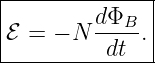
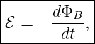
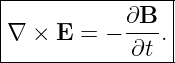
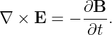
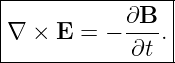
EM13 introduces the first fundamental mechanism that couples the electric and magnetic fields
dynamically:
Faraday’s law is one of the central experimental laws of Electromagnetism. In modern field
language it states that a time-varying magnetic field is associated with a circulating electric field.
This is a major conceptual step toward Maxwell’s equations, electromagnetic waves, radio
antennas, and RF receivers [1, 2, 3, 5].
1 Magnetic flux
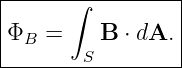
The magnetic flux through an oriented surface S is
The oriented area element is
where n is the chosen surface normal.
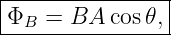
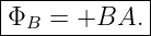
For a uniform magnetic field through a flat surface of area A,
where 𝜃 is the angle between B and the surface normal, not the surface itself.
The SI unit of magnetic flux is the weber:
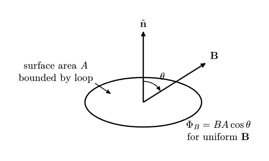
Figure. Magnetic flux through an oriented loop surface. The angle 𝜃 is measured between
B and the chosen normal n.
2 Electromotive force
The term electromotive force, abbreviated emf, is historical. An emf is not a mechanical force. It is
work done per unit charge around a circuit and therefore has units of volts.
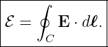
For a stationary closed contour C, the electric contribution to emf is
If the electric field were purely electrostatic, this closed-loop integral would vanish.
Electromagnetic induction introduces a different kind of electric field: one whose circulation around
a closed path can be nonzero.
3 Faraday’s law for a stationary loop
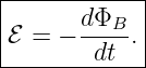
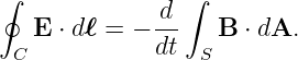
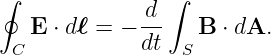
For a fixed loop and fixed spanning surface, Faraday’s law states
For a coil of N identical tightly coupled turns,
The negative sign is Lenz’s law. It encodes the direction of the induced emf relative to the chosen
loop orientation and magnetic-flux direction.
The magnetic flux can change because one or more of the following changes:
- the magnetic-field magnitude B;
- the area A of the loop;
- the orientation angle 𝜃;
- the spatial relationship between a nonuniform field and the loop.
4 Example 1: changing uniform magnetic field
A circular loop has radius
A uniform magnetic field normal to the loop increases from
to
in
The loop area is
Because the field is normal to the loop,
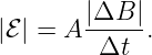
Thus,
| |ℰ| | = (2.01 × 10⁻²) | (15)
|
| = 2.01 × 10⁻² V. | (16) |
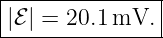
Therefore,
The sign and current direction require an orientation convention and Lenz’s law.
5 Lenz’s law
Lenz’s law gives a physical interpretation of the minus sign in Faraday’s law:
This does not mean the induced magnetic field always points opposite to the external magnetic
field. It opposes the change.
For example, if an external magnetic field into the page is increasing, an induced current produces
a magnetic field out of the page. If the same external field into the page is decreasing, the induced
response instead tends to maintain an into-page field.
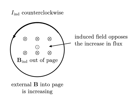
Figure. Lenz’s law for an increasing magnetic field into the page. The induced current is
counterclockwise so that its magnetic field points out of the page and opposes the increase
in inward flux.
6 Orientation conventions and the minus sign
The orientation of the loop and the orientation of the spanning surface are linked by the right-hand
rule.
If the fingers curl in the positive traversal direction around C, the thumb gives the positive normal
n. Magnetic flux is positive when B has a component along that normal.
With these linked orientations, the integral form of Faraday’s law for a stationary loop
is
The minus sign is therefore not an arbitrary extra rule. It is part of the oriented relationship
among the contour, surface normal, magnetic flux, and induced electric-field circulation.
7 Example 2: an N-turn coil
A coil has
turns and area per turn
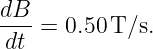
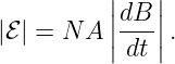
The field is normal to the coil and changes at the rate
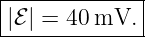
The emf magnitude is
| |ℰ| | = NA | (23)
|
| = (200)(4.0 × 10⁻⁴)(0.50) | (24)
|
| = 4.0 × 10⁻² V. | (25) |
Hence,
8 Rotating-loop induction
Suppose a loop of area A rotates in a uniform magnetic field B with angular speed ω. If the loop
normal makes angle
with the field, then
For an N-turn coil,
| ℰ | = −N [BA cos(ωt)] [BA cos(ωt)] | (29)
|
| = NBAω sin(ωt). | (30) |
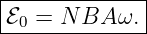
Therefore,
with peak emf
This is the idealized operating principle of an AC generator.
9 Example 3: rotating coil
Let
Then
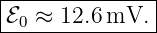
| ℰ0 | = (50)(1.0 × 10⁻²)(0.20)(100) | (34)
|
| = 10 V. | (35) |
Thus,
10 Motional emf
A changing magnetic flux can also occur because a Conductor moves through a magnetic
field.
A charge moving with conductor velocity v experiences the magnetic Lorentz force
The magnetic force per unit charge is
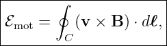
For a moving conductor, the motional contribution to emf is
where the relevant velocity is the velocity of the conductor element.
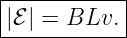
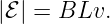
For a straight rod of length L moving with speed v perpendicular to both the rod and a uniform
magnetic field,
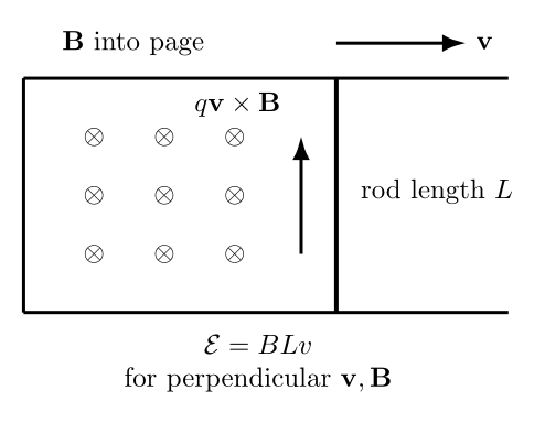
Figure. Motional emf in a sliding rod. The magnetic Lorentz force separates charge along
the moving conductor, producing an emf of magnitude BLv for the perpendicular geometry
shown.
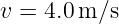
11 Example 4: sliding conducting rod
Let
Then
| |ℰ| | = BLv | (42)
|
| = (0.40)(0.50)(3.0) | (43)
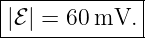
|
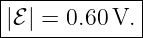
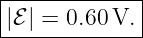
| = 0.60 V. | (44) |
Therefore,
12 Transformer emf and motional emf are physically distinct
Two mechanisms can contribute to circuit emf:
- Transformer emf: a time-varying magnetic field produces a circulating electric field
even when the circuit is stationary.
- Motional emf: magnetic Lorentz force acts on charges in a conductor moving through
a magnetic field.
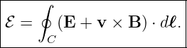
For a moving material circuit, the total Lorentz-force-per-charge circulation can be written
schematically as
Under the usual circuit conditions, this total emf is consistent with the flux rule
where the derivative includes changes caused by the field, the circuit geometry, or both.
However, the local Maxwell–Faraday equation introduced below refers specifically to the electric
field generated by a time-varying magnetic field. Keeping these mechanisms conceptually separate
prevents later confusion.
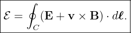
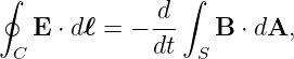
13 A changing magnetic field produces a circulating electric field
The field form of Faraday’s law does not require a conducting wire. A changing magnetic field can
produce an electric field in empty space.
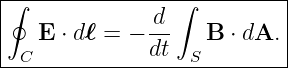
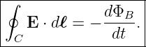
For a stationary closed contour C,
The induced electric field is generally not electrostatic. Its field lines can form closed loops, and its
closed-loop circulation can be nonzero.
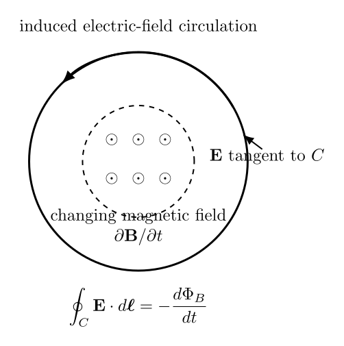
Figure. A changing magnetic field produces circulating electric-field lines. No physical
wire is required for the field law itself.
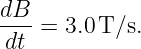
14 Example 5: induced electric field inside a changing-field region
Suppose a spatially uniform magnetic field occupies a circular region and changes at the rate
dB∕dt. Choose a circular observation contour of radius r lying completely inside that
region.
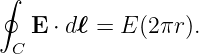
By rotational symmetry, the induced electric field is tangent to the circle and has constant
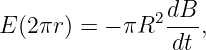
magnitude E(r). Therefore,
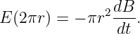
The enclosed magnetic flux is
Faraday’s law gives
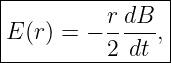
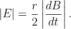
Thus,
where the sign denotes the circulation direction relative to the chosen contour orientation.
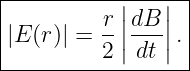
The magnitude is
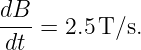
15 Example 6: induced electric field outside the changing-field region
Now suppose the changing magnetic field occupies only a circular region of radius R, while the
observation contour has radius r > R.
Only the field-containing area contributes to the magnetic flux:
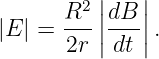
Therefore,
so
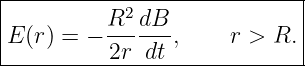
This field decreases as 1∕r outside the changing-flux region.
16 From integral Faraday law to the differential form
For a fixed contour and fixed spanning surface, Stokes’ theorem gives
Faraday’s law gives
For a fixed surface, the time derivative may be brought inside the surface integral:
Therefore,
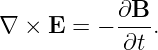
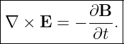
For arbitrary surfaces,
This is the Maxwell–Faraday equation.
It connects directly back to the curl operator introduced in EM03. Curl is no longer merely a
mathematical measure of local circulation: in electromagnetism, the curl of the electric field is tied
directly to the local time variation of the magnetic field.
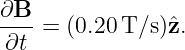
17 Example 7: interpreting the differential equation
Suppose at some point in space
Then Maxwell–Faraday gives
Thus the local electric-field circulation has negative z orientation. Using the right-hand rule, that
corresponds to clockwise local circulation when viewed from the +z side.
18 Why Lenz’s law is required by energy conservation
Suppose the induced current reinforced the change in magnetic flux rather than opposing it. An
increasing flux would produce a current that created still more flux in the same direction, which
would drive still more current. The system would amplify itself without an external energy
source.
Lenz’s law prevents that unphysical behavior. Mechanical work or another energy source is
required to change the flux against the induced response.
For the sliding rod, for example, the induced current experiences a magnetic force opposing the
imposed motion. To maintain constant speed, an external agent must do mechanical work. That
mechanical power can appear as electrical power and ultimately as resistive heating in the
circuit.
19 A first bridge to antennas and radio waves
Faraday’s law is one of the equations that makes electromagnetic waves possible. A time-varying
magnetic field produces a circulating electric field:
Later, Maxwell’s correction to Ampère’s law will show the complementary relationship: a
time-varying electric field contributes to the curl of the magnetic field.
Together, these coupled curl equations allow electric and magnetic disturbances to propagate
through space as electromagnetic waves.
The induction viewpoint is also directly relevant to receiving antennas. A time-varying
electromagnetic field can induce voltage and current in a conducting structure. The exact RF
antenna problem requires the full Maxwell theory developed later, but Faraday’s law provides one
of the fundamental pieces.
20 Common mistakes
- Mistake: measuring 𝜃 from the plane of the loop rather than from its normal. In
ΦB = BA cos 𝜃, 𝜃 is the angle between B and n.
- Mistake: saying that Lenz’s law opposes the magnetic field. It opposes the change in
magnetic flux.
- Mistake: treating emf as a mechanical force. Emf has units of volts and represents
work per unit charge.
- Mistake: assuming that a wire is required for an induced electric field. The
Maxwell–Faraday field equation exists in space whether or not a conductor is present.
- Mistake: using BLv without checking that the rod, velocity, and magnetic field have
the required perpendicular geometry.
- Mistake: mixing motional emf and transformer emf without recognizing their different
local force mechanisms.
- Mistake: applying the simple stationary-contour integral form without considering
whether the circuit itself is moving or deforming.
Part I: Exercises
All exercises are stated here before any worked solution. Attempt the complete set before
proceeding to Part II.
Exercise 1: magnetic flux through a tilted loop
A uniform magnetic field has magnitude
A flat loop has area
and its area normal makes an angle
with the magnetic field. Find the magnetic flux.
Exercise 2: flux sign and orientation
A loop has area A and a magnetic field of magnitude B points exactly opposite to the chosen area
normal.
Find the signed magnetic flux and explain what happens to the sign if the area-normal convention
is reversed.
Exercise 3: induced emf from a changing field
A single-turn loop has area
A perpendicular magnetic field increases uniformly from 0.20 T to 0.50 T in 0.10 s. Find the emf
magnitude.
Exercise 4: multiturn coil
A 150-turn coil has area per turn
A perpendicular magnetic field decreases at the constant rate
Find the induced emf magnitude.
Exercise 5: Lenz-law direction
A circular conducting loop is viewed face-on. An external magnetic field points out of the page and
is increasing.
Determine:
- the direction of the induced magnetic field;
- whether the induced current is clockwise or counterclockwise.
Exercise 6: rotating-loop generator
A 40-turn coil of area
rotates at angular speed
in a uniform magnetic field
Find the peak induced emf.
Exercise 7: motional emf
A conducting rod of length
moves at speed
perpendicular to a uniform field
The rod is perpendicular to both v and B. Find the motional emf magnitude.
Exercise 8: magnetic force direction in a moving rod
A conducting rod moves in the +x direction through a magnetic field in the −z direction.
For a positive charge moving with the rod, find the direction of
Which end of a rod oriented along the y axis tends to become positively charged?
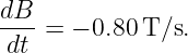
Exercise 9: induced electric field inside a changing-field region
A uniform magnetic field fills a circular region and changes at the rate
Find the magnitude of the induced electric field on a circular contour of radius
lying entirely inside the changing-field region.
Exercise 10: induced electric field outside a changing-field region
A uniform changing magnetic field occupies a circular region of radius
and changes at the rate
Find the induced electric-field magnitude at radius
Exercise 11: derive the differential Maxwell–Faraday equation
Starting from
for a fixed contour and surface, use Stokes’ theorem to derive
Exercise 12: energy and Lenz’s law
Explain why an induced current that reinforced the flux change that produced it would conflict
with energy conservation. Use either a moving magnet and loop or a sliding conducting rod as your
physical example.
Exercise 13: transformer emf versus motional emf
For each case below, identify the primary local mechanism producing emf:
- a stationary wire loop in a time-varying magnetic field;
- a conducting rod moving through a static magnetic field;
- a moving loop in a magnetic field that is also changing with time.
State which cases can contain an electric-field contribution, a v × B contribution, or
both.
Exercise 14: RF loop preview
A single-turn receiving loop has area
A locally uniform sinusoidal magnetic field normal to the loop is
with
Ignoring loading and radiation effects, find:
- an expression for the induced emf ℰ(t);
- the peak emf magnitude.
Part II: Complete Worked Solutions
Solution 1: magnetic flux through a tilted loop
For a uniform field through a flat area,
Substitute the values:
| ΦB | = (0.35)(2.0 × 10⁻²) cos 60∘ | (89)
|
| = (0.35)(2.0 × 10⁻²)(0.5) | (90)
|
| = 3.5 × 10⁻³ Wb. | (91) |
Therefore,
Solution 2: flux sign and orientation
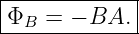
If B points opposite to the chosen normal, then
Therefore,
So
If the area-normal convention is reversed, the same physical field now points along the positive
normal and the signed flux becomes
The physical configuration has not changed; only the orientation convention has changed.
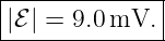
Solution 3: induced emf from a changing field
The field change is
The emf magnitude is
| |ℰ| | = A | (98)
|
| = (3.0 × 10⁻³) | (99)
|
| = 9.0 × 10⁻³ V. | (100) |
Thus,
Solution 4: multiturn coil
For N turns,
Hence,
| |ℰ| | = (150)(5.0 × 10⁻⁴)(0.80) | (103)
|
| = 6.0 × 10⁻² V. | (104) |
Therefore,
Solution 5: Lenz-law direction
The external field points out of the page and is increasing. The induced response opposes the
increase, so the induced magnetic field must point into the page.
Thus,
Using the right-hand rule, a clockwise current produces a magnetic field into the page.
Therefore,
Solution 6: rotating-loop generator
The peak emf is
Substitute:
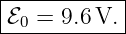
| ℰ0 | = (40)(0.25)(8.0 × 10⁻³)(120) | (109)
|
| = 9.6 V. | (110) |
Therefore,
Solution 7: motional emf
For the perpendicular sliding-rod geometry,
Hence,
| |ℰ| | = (0.50)(0.30)(4.0) | (113)
|
| = 0.60 V. | (114) |
Thus,
Solution 8: magnetic force direction in a moving rod
The rod velocity is
and the field is
Therefore,
| v × B | ∝x × (−z) | (118)
|
| = −x ×z | (119)
|
| = +y. | (120) |
For a positive charge,
So the +y end of a rod oriented along the y axis tends to become positively charged.
Solution 9: induced electric field inside a changing-field region
Inside the changing-field region,
Substitute:
| |E| | = 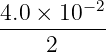 (3.0) (3.0) | (123)
|
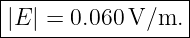
| = 6.0 × 10⁻² V/m. | (124) |
Therefore,
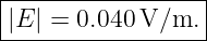
Solution 10: induced electric field outside a changing-field region
For r > R,
Substitute:
| |E| | =  (2.5) (2.5) | (127)
|
| = 4.0 × 10⁻² V/m. | (128) |
Hence,
Solution 11: derive the differential Maxwell–Faraday equation
Start with the stationary-contour integral form:
Apply Stokes’ theorem to the left-hand side:
For a fixed surface,
Therefore,
Because this holds for arbitrary fixed surfaces,
Solution 12: energy and Lenz’s law
Suppose an induced current reinforced the change in flux. If a magnet approached a conducting
loop, the increasing flux would induce a current whose magnetic field increased the flux further.
That stronger change would induce an even larger current, producing self-amplification without a
corresponding energy input.
Instead, the induced current creates a magnetic effect that resists the imposed change. An external
agent must therefore do work to continue moving the magnet or conductor. That work supplies the
electrical energy that may later be dissipated as heat or stored in the electromagnetic
system.
Thus Lenz’s law is consistent with energy conservation:
Solution 13: transformer emf versus motional emf
- A stationary loop in a time-varying magnetic field has a transformer emf. The
local mechanism is a nonconservative induced electric field, represented by E in the
circulation integral.
- A rod moving through a static magnetic field has a motional emf. The local
mechanism is the magnetic Lorentz force per unit charge, v × B.
- A moving loop in a field that also varies in time may have both contributions. The
total emf may include both E and v × B terms.
Thus the general circuit-force-per-charge viewpoint is
Solution 14: RF loop preview
The magnetic field is
Because the field is normal to the loop,
Faraday’s law gives
| ℰ(t) | = − | (139)
|
| = 2πfAB0 sin(2πft). | (140) |
Therefore,
The peak magnitude is
Using
we obtain
| ℰ0 | = 2π(1.0 × 10⁶)(1.0 × 10⁻⁴)(20 × 10−6) | (144)
|
| = 1.26 × 10⁻² V. | (145) |
Hence,
This simple result is only a preview. A practical RF loop antenna must also be treated using
circuit loading, self-inductance, impedance, radiation, field polarization, and the full Maxwell
equations.
21 What EM13 adds to the series
EM12 established the magnetostatic curl relation
EM13 adds the first explicitly time-dependent field coupling:
The next major step is to complete Ampère’s law with Maxwell’s displacement-current term.
Once both curl equations contain time-dependent field terms, the mathematical structure needed
for self-propagating electromagnetic waves is nearly complete.
References
[1] David J. Griffiths, Introduction to Electrodynamics, 4th ed., Cambridge University
Press, 2017.
[2] Edward M. Purcell and David J. Morin, Electricity and Magnetism, 3rd ed.,
Cambridge University Press, 2013.
[3] Samuel J. Ling, Jeff Sanny, and William Moebs, University Physics, Volume 2,
OpenStax, 2016, sections on electromagnetic induction, Faraday’s law, motional emf, and
generators.
[4] Richard P. Feynman, Robert B. Leighton, and Matthew Sands, The Feynman Lectures
on Physics, Volume II, Addison-Wesley, 1964, chapters on induction and Maxwell’s
equations.
[5] Massachusetts Institute of Technology, 8.02 Physics II: Electricity and Magnetism,
MIT OpenCourseWare, materials on magnetic flux, Faraday’s law, Lenz’s law, motional
emf, and induction.